Discplined Convex Programming
Disciplined convex programming (DCP) is a system for constructing
mathematical expressions with known curvature from a given library of
base functions. CVXR uses DCP to ensure that the specified
optimization problems are convex.
This section of the tutorial explains the rules of DCP and how they
are applied by CVXR.
Visit dcp.stanford.edu for a more interactive introduction to DCP.
Expressions
Expressions in CVXR are formed from variables, numerical
constants such as R vectors and matrices, the standard
arithmetic operators +, -, *, %*%, /, and a library
of functions. Here are some examples of
CVXR expressions:
suppressWarnings(suppressMessages(library(CVXR)))
## Create variables.
x <- Variable()
y <- Variable()
## Examples of cvxr expressions.
3.69 + x / 3
## AddExpression(c("list() / 3", "varNA / 3"), 3.69)x - 4 * y## AddExpression(varNA, c("-list() * varNA", "-4 * varNA"))sqrt(x) - min_elemwise(y, x - 2.5)## AddExpression(Power(varNA, 1/2), -MinElemwise(varNA, varNA + -2.5))max_elemwise(2.66 - sqrt(y), abs(x + 2 * y))## MaxElemwise(-Power(varNA, 1/2) + 2.66, Abs(varNA + c("list() * varNA", "2 * varNA")))Expressions can be scalars, vectors, or matrices. The dimensions of an
expression can be obtained using the function size. CVXR will
raise an exception if an expression is used in a way that doesn’t make
sense given its dimensions, e.g. adding matrices of different
sizes.
Z <- Variable(5, 4)
A <- matrix(1, nrow = 2, ncol = 5)

## Use size to get the dimensions.
cat("dimensions of Z:", size(Z), "\n")
## dimensions of Z: 20cat("dimensions of sum_entries(Z):", size(sum_entries(Z)), "\n")## dimensions of sum_entries(Z): 1cat("dimensions of A %*% Z:", size(A %*% Z), "\n")## dimensions of A %*% Z: 8Error raised for invalid dimensions.
tryCatch(A + Z, error = function(e) geterrmessage())## [1] "Cannot broadcast dimensions"CVXR uses DCP analysis to determine the sign and curvature of each
expression.
Sign
Each (sub)expression is flagged as positive (non-negative), negative (non-positive), zero, or unknown.
The signs of larger expressions are determined from the signs of their
subexpressions. For example, the sign of the expression expr1 * expr2 is
- Zero if either expression has sign zero.
- Positive if
expr1andexpr2have the same (known) sign. - Negative if
expr1andexpr2have opposite (known) signs. - Unknown if either expression has unknown sign.
The sign given to an expression is always correct. However, DCP sign analysis
may flag an expression as unknown sign when the sign could be figured
out through more complex analysis. For instance, x * x is positive but
has unknown sign by the rules above.
CVXR determines the sign of constants by looking at their value. For
scalar constants, this is straightforward. Vector and matrix constants
with all positive (negative) entries are marked as positive
(negative). Vector and matrix constants with both positive and
negative entries are marked as unknown sign.
The sign of an expression is obtained via the sign function:
x <- Variable()
a <- Constant(-1)
c <- matrix(c(1, -1), ncol = 1)

cat("sign of x:", sign(x), "\n")
## sign of x: UNKNOWNcat("sign of a:", sign(a), "\n")## sign of a: NONPOSITIVEcat("sign of abs(x):", sign(abs(x)), "\n")## sign of abs(x): NONNEGATIVEcat("sign of c*a:", sign(c * a), "\n")## sign of c*a: UNKNOWNCurvature
Each (sub)expression is flagged as one of the following curvatures (with respect to its variables)
| Curvature | Meaning |
|---|---|
| constant | f(x) independent of x |
| affine | f(θx+(1−θ)y)=θf(x)+(1−θ)f(y),∀x,y,θ∈[0,1] |
| convex | f(θx+(1−θ)y)≤θf(x)+(1−θ)f(y),∀x,y,θ∈[0,1] |
| concave | f(θx+(1−θ)y)≥θf(x)+(1−θ)f(y),∀x,y,θ∈[0,1] |
| unknown | DCP analysis cannot determine the curvature |
using the curvature rules given below. As with sign analysis, the conclusion is always correct, but the simple analysis can flag expressions as unknown even when they are convex or concave. Note that any constant expression is also affine, and any affine expression is convex and concave.
Curvature rules
DCP analysis is based on applying a general composition theorem from convex analysis to each (sub)expression.
f(e1,e2,…,en) is convex if f is a convex function and for each ei, one of the following conditions holds:
- f is increasing in argument i and ei is convex.
- f is decreasing in argument i and ei is concave.
- ei is affine or constant.
f(e1,e2,…,en) is concave if f is a concave function and for each ei one of the following conditions holds:
- f is increasing in argument i and ei is concave.
- f is decreasing in argument i and ei is convex.
- ei is affine or constant.
f(e1,e2,…,en) is affine if f is an affine function and each ei is affine.
If none of the three rules apply, the expression f(e1,e2,…,en) is marked as having unknown curvature.
Whether a function is increasing or decreasing in an argument may depend
on the sign of the argument. For instance, abs is increasing for
positive arguments and decreasing for negative arguments.
The curvature of an expression is determined using the curvature
function:
x <- Variable()
a <- Constant(5)

cat("curvature of x:", curvature(x), "\n")
## curvature of x: AFFINEcat("curvature of a:", curvature(a), "\n")## curvature of a: CONSTANTcat("curvature of abs(x):", curvature(abs(x)), "\n")## curvature of abs(x): CONVEXcat("curvature of sqrt(x):", curvature(sqrt(x)), "\n")## curvature of sqrt(x): CONCAVEInfix operators
The infix operators +, -, *, %*%, / are treated exactly like functions.
The infix operators + and - are affine, so the rules above are
used to flag the curvature. For example, expr1 + expr2 is flagged as
convex if expr1 and expr2 are convex.
expr1*expr2 and expr1 %*% expr2 are allowed only when one of the expressions is constant.
If both expressions are non-constant, CVXR will raise an exception.
expr1/expr2 is allowed only when expr2 is a scalar constant. The
curvature rules above apply. For example, expr1/expr2 is convex when
expr1 is concave and expr2 is negative and constant.
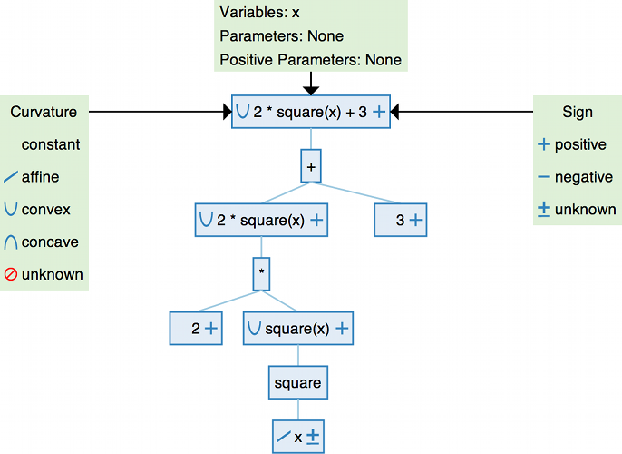
Example 1
DCP analysis breaks expressions down into subexpressions. The tree
visualization below shows how this works for the expression
2*square(x) + 3. Here square is synonymous with squaring each element of the input x.
Each subexpression is displayed in a blue box. We mark its curvature on the left and its sign on the right.
Example 2
We’ll walk through the application of the DCP rules to the expression
sqrt(1 + square(x)).
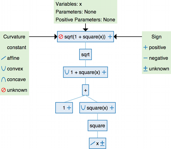
The variable x has affine curvature and unknown sign. The square
function is convex and non-monotone for arguments of unknown sign. It
can take the affine expression x as an argument; the result
square(x) is convex.
The arithmetic operator + is affine and increasing, so the
composition 1 + square(x) is convex by the curvature rule for convex
functions. The function sqrt is concave and increasing, which means
it can only take a concave argument. Since 1 + square(x) is convex,
sqrt(1 + square(x)) violates the DCP rules and cannot be verified as
convex.
In fact, sqrt(1 + square(x)) is a convex function of x, but the
DCP rules are not able to verify convexity. If the expression is
written as p_norm(vstack(1, x), 2), the l2 norm of the vector [1,x],
which has the same value as sqrt(1 + square(x)), then it will be
certified as convex using the DCP rules.
cat("sqrt(1 + square(x)) curvature:", curvature(sqrt(1 + square(x))), "\n")## sqrt(1 + square(x)) curvature: UNKNOWNcat("p_norm(vstack(1, x), 2) curvature:", curvature(p_norm(vstack(1, x), 2)), "\n")## p_norm(vstack(1, x), 2) curvature: CONVEXDCP problems
A problem is constructed from an objective and a list of constraints. If
a problem follows the DCP rules, it is guaranteed to be convex and
solvable by CVXR. The DCP rules require that the problem objective have
one of two forms:
- Minimize(convex)
- Maximize(concave)
The only valid constraints under the DCP rules are
- affine == affine
- convex <= concave
- concave >= convex
You can check that a problem, constraint, or objective satisfies the DCP
rules by calling is_dcp(object). Here are some examples of DCP and
non-DCP problems:
x <- Variable()
y <- Variable()

## DCP problems.
prob1 <- Problem(Minimize((x - y)^2), list(x + y >= 0))
prob2 <- Problem(Maximize(sqrt(x - y)),
                 list(2 * x - 3 == y,
                      x^2 <= 2))

cat("prob1 is DCP:", is_dcp(prob1), "\n")
## prob1 is DCP: TRUEcat("prob2 is DCP:", is_dcp(prob2), "\n")## prob2 is DCP: TRUE## Non-DCP problems.
## A non-DCP objective.
prob3 <- Problem(Maximize(x^2))
cat("prob3 is DCP:", is_dcp(prob3), "\n")## prob3 is DCP: FALSEcat("Maximize(x^2) is DCP:", is_dcp(Maximize(x^2)), "\n")## Maximize(x^2) is DCP: FALSE## A non-DCP constraint.
prob4 <- Problem(Minimize(x^2), list(sqrt(x) <= 2))
cat("prob4 is DCP:", is_dcp(prob4), "\n")## prob4 is DCP: FALSEcat("sqrt(x) <= 2 is DCP:", is_dcp(sqrt(x) <= 2), "\n")## sqrt(x) <= 2 is DCP: FALSECVXR will raise an exception if you call solve() on a non-DCP
problem.
## A non-DCP problem.
prob <- Problem(Minimize(sqrt(x)))
tryCatch(solve(prob), error = function(e) geterrmessage())
## [1] "Problem does not follow DCP rules."Session Info
sessionInfo()## R version 4.4.2 (2024-10-31)
## Platform: x86_64-apple-darwin20
## Running under: macOS Sequoia 15.1
##
## Matrix products: default
## BLAS: /Library/Frameworks/R.framework/Versions/4.4-x86_64/Resources/lib/libRblas.0.dylib
## LAPACK: /Library/Frameworks/R.framework/Versions/4.4-x86_64/Resources/lib/libRlapack.dylib; LAPACK version 3.12.0
##
## locale:
## [1] en_US.UTF-8/en_US.UTF-8/en_US.UTF-8/C/en_US.UTF-8/en_US.UTF-8
##
## time zone: America/Los_Angeles
## tzcode source: internal
##
## attached base packages:
## [1] stats graphics grDevices datasets utils methods base
##
## other attached packages:
## [1] kableExtra_1.4.0 CVXR_1.0-15
##
## loaded via a namespace (and not attached):
## [1] gmp_0.7-5 clarabel_0.9.0.1 sass_0.4.9 xml2_1.3.6
## [5] slam_0.1-54 blogdown_1.19 stringi_1.8.4 lattice_0.22-6
## [9] digest_0.6.37 magrittr_2.0.3 evaluate_1.0.1 grid_4.4.2
## [13] bookdown_0.41 fastmap_1.2.0 jsonlite_1.8.9 Matrix_1.7-1
## [17] Rmosek_10.2.0 viridisLite_0.4.2 scales_1.3.0 codetools_0.2-20
## [21] jquerylib_0.1.4 cli_3.6.3 Rmpfr_0.9-5 rlang_1.1.4
## [25] Rglpk_0.6-5.1 bit64_4.5.2 munsell_0.5.1 cachem_1.1.0
## [29] yaml_2.3.10 tools_4.4.2 Rcplex_0.3-6 rcbc_0.1.0.9001
## [33] colorspace_2.1-1 gurobi_11.0-0 assertthat_0.2.1 vctrs_0.6.5
## [37] R6_2.5.1 lifecycle_1.0.4 stringr_1.5.1 bit_4.5.0
## [41] cccp_0.3-1 bslib_0.8.0 glue_1.8.0 Rcpp_1.0.13-1
## [45] systemfonts_1.1.0 xfun_0.49 highr_0.11 rstudioapi_0.17.1
## [49] knitr_1.48 htmltools_0.5.8.1 rmarkdown_2.29 svglite_2.1.3
## [53] compiler_4.4.2