A Gentle Introduction to `CVXR`
Introduction
Welcome to CVXR: a modeling language for describing and solving
convex optimization problems that follows the natural, mathematical
notation of convex optimization rather than the requirements of any
particular solver. The purpose of this document is both to introduce
the reader to CVXR and to generate excitement for its possibilities in
the field of statistics.
Convex optimization is a powerful and very general tool. As a practical matter, the set of convex optimization problems includes almost every optimization problem that can be solved exactly and efficiently (i.e. without requiring an exhaustive search). If an optimization problem can be solved, it is probably convex. This family of problems becomes even larger if you include those that can be solved approximately and efficiently. To learn more about the mathematics and applications of convex optimization, see Boyd and Vandenberghe 2009.
Convex optimization systems written in other languages are already
widely used in practical applications. These
include
YALMIP and
CVX
(Matlab), CVXPY (Python),
and Convex.jl
(Julia). CVXR Shares a lot of its code base
with
CVXcanon and
CVXPY. As far as we know, this is the first full-featured general
convex optimization package for R.
One of the great headaches of conventional numerical optimization is
the process of deciding which algorithm to use and how to set its
parameters. In convex optimization, the particular algorithm matters
much less. So while a user of CVXR is still free to choose from a
number of different algorithms and to set algorithm parameters as they
please, the vast majority of users will not need to do this. CVXR
will just work.
The uses for convex optimization in statistics are many and varied. A large number of parameter-fitting methods are convex, including least-squares, ridge, lasso, and isotonic regression, as well as many other kinds of problems such as maximum entropy or minimum Kullback-Leibler divergence over a finite set.
All of these examples, at least in their most basic forms, are
established enough that they already have well-crafted R packages
devoted to them. If you use CVXR to solve these problems, it will
work. It will probably be slower than a custom-built algorithm—for
example, glmnet for fitting lasso or ridge regression models—but it
will work. However, this is not the true purpose of CVXR. If you
want to build a well-established model, you should use one of the
well-established packages for doing so. If you want to build your
own model—one that is a refinement of an existing method, or
perhaps even something that has never been tried before—then CVXR
is the package to do it. The advantage of CVXR over glmnet and the
like comes from its flexibility: A few lines of code can transform a
problem from commonplace to state-of-the-art, and can often do the
work of an entire package in the process.
This document is meant to familiarize you with the CVXR package. It
assumes basic knowledge of convex optimization and statistics as well
as proficiency with R. A potential user of CVXR should read this entire
document and then refer to the tutorial examples.
Happy optimizing!
Convex Optimization
A convex optimization problem has the following form:
\[ \begin{array}{ll} \mbox{minimize} & f_0(x)\\ \mbox{subject to} & f_i(x) \leq 0, \quad i=1,\ldots,m\\ & g_i(x) = 0, \quad i=1,\ldots,p \end{array} \]
where \(x\) is the variable, \(f_0\) and \(f_1,...,f_m\) are convex, and \(g_1,...,g_p\) are affine. \(f_0\) is called the objective function, \(f_i \leq 0\) are called the inequality constraints, and \(g_i = 0\) are called the equality constraints.
In CVXR, you will specify convex optimization problems in a more
convenient format than the one above.
A convex function is one that is upward curving. A concave function is downward curving. An affine function is flat, and is thus both convex and concave.
A convex optimization problem is one that attempts to minimize a convex function (or maximize a concave function) over a convex set of input points.
You can learn much more about convex optimization via Boyd and Vandenberghe (2004) as well as the CVX101 MOOC.
‘Hello World’
We begin with one of the simplest possible problems that presents all three of these features:
\[ \begin{array}{ll} \mbox{minimize} & x^2 + y^2 \\ \mbox{subject to} & x \geq 0, \quad 2x + y = 1 \end{array} \]
with scalar variables \(x\) and \(y\). This is a convex optimization problem with objective \(f_0(x,y) = x^2 + y^2\) and constraint functions \(f_1(x,y) = -x\) and \(g_1(x,y) = 2x - y - 1\).
Note that this problem is simple enough to be solved analytically, so
we can confirm that CVXR has produced the correct answer. Here’s how
we formulate the problem in CVXR.
# Variables minimized over
x <- Variable(1)
y <- Variable(1)

# Problem definition
objective <- Minimize(x^2 + y^2)
constraints <- list(x >= 0, 2*x + y == 1)
prob2.1 <- Problem(objective, constraints)

# Problem solution
solution2.1 <- solve(prob2.1)
solution2.1$status
## [1] "optimal"solution2.1$value## [1] 0.2solution2.1$getValue(x)## [1] 0.4solution2.1$getValue(y)## [1] 0.2# The world says 'hi' back.We now turn to a careful explanation of the code. The first lines
create two Variable objects, x and y, both of length 1
(i.e. scalar variables).
x <- Variable(1)
y <- Variable(1)
x and y represent what we are allowed to adjust in our problem in
order to obtain the optimal solution. They don’t have values yet, and
they won’t until after we solve the problem. For now, they are just
placeholders.
Next, we define the problem objective.
objective <- Minimize(x^2 + y^2)This call to Minimize() does not return the minimum value of the
expression x^2 + y^2 the way a call to the native R function min()
would do (after all, x and y don’t have values yet). Instead,
Minimize() creates an Objective object, which defines the goal of
the optimization we will perform, namely to find values for x and
y which produce the smallest possible value of x^2 + y^2.
The next line defines two constraints—an inequality constraint and an equality constraint, respectively.
constraints <- list(x >= 0, 2*x + y == 1)Again, counter to what you might ordinarily expect, the expression x >= 0 does not return TRUE or FALSE the way 1.3 >= 0
would. Instead, the == and >= operators have been overloaded to
return Constraint objects, which will be used by the solver to enforce
the problem’s constraints. (Without them, the solution to our problem
would simply be \(x = y = 0\).)
Next, we define our Problem object, which takes our Objective object and our two Constraint objects as inputs.
prob2.1 <- Problem(objective, constraints)Problem objects are very flexible in that they can have 0 or more
constraints, and their objective can be to Minimize() a convex
expression (as shown above) or to Maximize() a concave
expression.
The call to Problem() still does not actually solve our
optimization problem. That only happens with the call to solve().
solution2.1 <- solve(prob2.1)Behind the scenes, this call translates the problem into a format that
a convex solver can understand, feeds the problem to the solver, and
then returns the results in a list. For this problem, the
list will contain among other things the optimal value of
the objective function x^2 + y^2, values for x and y that
achieve that optimal objective value (along with a function
solution2.1$getValue to retrieve them conveniently), and some
accompanying metadata such as solution2.1$status, which confirms
that the solution was indeed "optimal".
solution2.1$status## [1] "optimal"solution2.1$value## [1] 0.2solution2.1$getValue(x)## [1] 0.4solution2.1$getValue(y)## [1] 0.2In general, when you apply the solve() method to a Problem, several
things can happen:
solution$status == "optimal": The problem was solved. Values for the optimization variables were found, which satisfy all of the constraints and minimize/maximize the objective.solution$status == "infeasible": The problem was not solved because no combination of input variables exists that can satisfy all of the constraints. For a trivial example of when this might happen, consider a problem with optimization variablex, and constraintsx >= 1andx <= 0. Obviously, no value ofxexists that can satisfy both constraints. In this case,solution$valueis+Inffor a minimization problem and-Inffor a maximization problem, indicating infinite dissatisfaction with the result. The values for the input variables areNA.solution$status == "unbounded": The problem was not solved because the objective can be made arbitrarily small for a minimization problem or arbitrarily large for a maximization problem. Hence there is no optimal solution because for any given solution, it is always possible to find something even more optimal. In this case,solution$opt.valis-Inffor a minimization problem and+Inffor a maximization problem, indicating infinite satisfaction with the result. Again, the values of the the input variables areNA.
Modifying a CVXR Problem
Like any normal R object, the Problem, Minimize, Maximize, and
Constraint objects can all be modified and computed upon after
creation. Here is an example where we modify the problem we created
above by changing its objective and adding a constraint, print the
modified problem, check whether it is still convex, and then solve the
modified problem:
# Modify the problem from example 1
prob2.2 <- prob2.1
objective(prob2.2) <- Minimize(x^2 + y^2 + abs(x-y))
constraints(prob2.2) <- c(constraints(prob2.1), y <= 1)

# Solve the modified problem
solution2.2 <- solve(prob2.2)

# Examine the solution
solution2.2$status
## [1] "optimal"solution2.2$value## [1] 0.2222222solution2.2$getValue(x)## [1] 0.3333333solution2.2$getValue(y)## [1] 0.3333333An Invalid Problem
Unfortunately, you can’t just type any arbitrary problem you like into
CVXR. There are restrictions on what kinds of problems can be
handled. For example, if we tried to `Maximize()’ the objective from
example 2.1, we get an error:
prob2.3 <- prob2.1
objective(prob2.3) <- Maximize(x^2 + y^2)
solve(prob2.3)
## Error in construct_intermediate_chain(object, candidate_solvers, gp = gp): Problem does not follow DCP rules.We would get a similar error if we tried to add the constraint
p_norm(x,2) == 1. This is because CVXR uses a strict set of rules
called Disciplined Convex Programming (DCP) to evaluate the convexity
of any given problem. If you follow these rules, you are guaranteed
that your problem is convex. If you don’t follow these rules, CVXR
will throw an exception. See the last section for further information
on DCP.
Simple Examples
We begin by showing what a standard linear regression problem looks
like in CVXR:
Ordinary Least Squares
For illustration, we generate some synthetic data for use in this example.
set.seed(1)
s <- 1
n <- 10
m <- 300
mu <- rep(0, 9)
Sigma <- cbind(c(1.6484, -0.2096, -0.0771, -0.4088, 0.0678, -0.6337, 0.9720, -1.2158, -1.3219),
               c(-0.2096, 1.9274, 0.7059, 1.3051, 0.4479, 0.7384, -0.6342, 1.4291, -0.4723),
               c(-0.0771, 0.7059, 2.5503, 0.9047, 0.9280, 0.0566, -2.5292, 0.4776, -0.4552),
               c(-0.4088, 1.3051, 0.9047, 2.7638, 0.7607, 1.2465, -1.8116, 2.0076, -0.3377),
               c(0.0678, 0.4479, 0.9280, 0.7607, 3.8453, -0.2098, -2.0078, -0.1715, -0.3952),
               c(-0.6337, 0.7384, 0.0566, 1.2465, -0.2098, 2.0432, -1.0666,  1.7536, -0.1845),
               c(0.9720, -0.6342, -2.5292, -1.8116, -2.0078, -1.0666, 4.0882,  -1.3587, 0.7287),
               c(-1.2158, 1.4291, 0.4776, 2.0076, -0.1715, 1.7536, -1.3587, 2.8789, 0.4094),
               c(-1.3219, -0.4723, -0.4552, -0.3377, -0.3952, -0.1845, 0.7287, 0.4094, 4.8406))

X <- MASS::mvrnorm(m, mu, Sigma)
X <- cbind(rep(1, m), X)
trueBeta <- c(0, 0.8, 0, 1, 0.2, 0, 0.4, 1, 0, 0.7)
y <- X %*% trueBeta + rnorm(m, 0, s)
beta <- Variable(n)
objective <- Minimize(sum_squares(y - X %*% beta))
prob3.1 <- Problem(objective)Here, y is the response, X is the matrix of predictors, n is the
number of predictors, and beta is a vector of coefficients on the
predictors. The Ordinary Least-Squares (OLS) solution for beta
minimizes the \(l_2\)-norm of the residuals (i.e. the
root-mean-squared error). As we can see below, CVXR’s solution
matches the solution obtained by using lm.
CVXR_solution3.1 <- solve(prob3.1)
lm_solution3.1 <- lm(y ~ 0 + X)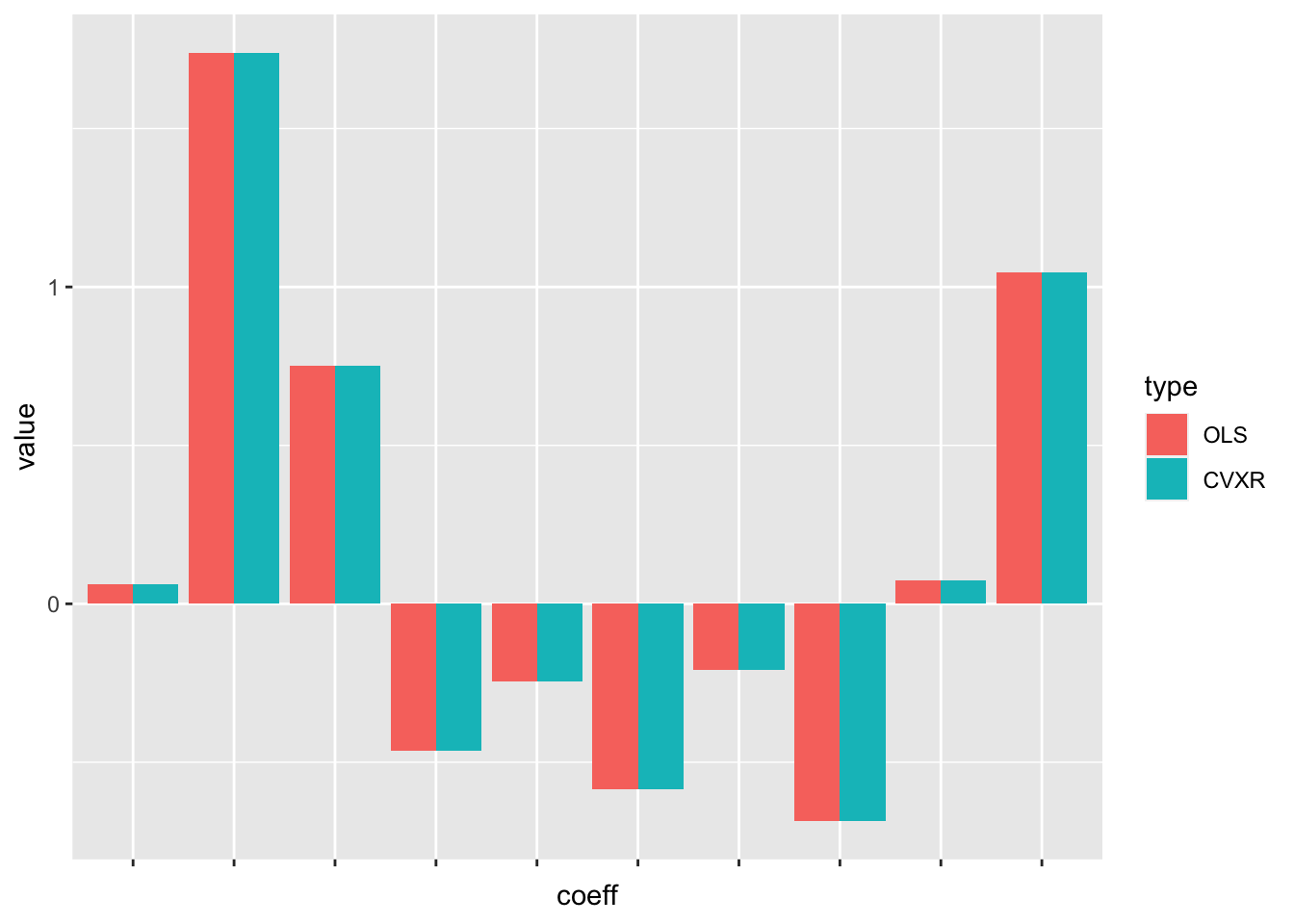
Obviously, if all you want to do is least-squares linear regression,
you should simply use lm. The chief advantage of CVXR is its
flexibility, as we will demonstrate in the rest of this section.
Non-Negative Least Squares
Looking at example 3.1, you may notice that the OLS regression problem
has an objective, but no constraints. In many contexts, we can greatly
improve our model by constraining the solution to reflect our prior
knowledge. For example, we may know that the coefficients beta must
be non-negative.
prob3.2 <- prob3.1
constraints(prob3.2) <- list(beta >= 0)
solution3.2 <- solve(prob3.2)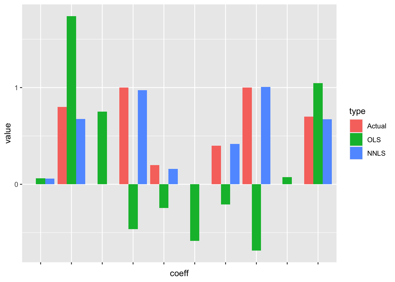
As we can see in the figure above, adding that one constraint produced a massive improvement in the accuracy of the estimates. Not only are the non-negative least-squares estimates much closer to the true coefficients than the OLS estimates, they have even managed to recover the correct sparsity structure in this case.
Like with OLS, there are already R packages available which implement
non-negative least squares, such as nnls. But that is
actually an excellent demonstration of the power of CVXR: A single
line of code here, namely prob3.2$constraints <- list(beta >= 0), is
doing the work of an entire package.
Support Vector Classifiers
Another common statistical tool is the support vector classifier (SVC). The SVC is an affine function (hyperplane) that separates two sets of points by the widest margin. When the sets are not linearly separable, the SVC is determined by a trade-off between the width of the margin and the number of points that are misclassified.
For the binary case, where the response \(y_i \in \{-1,1\}\), the SVC is obtained by solving
\[ \begin{array}{ll} \mbox{minimize} & \frac{1}{2}\Vert\beta\Vert^2 + C\sum_{i=1}^m \xi_i \\ \mbox{subject to} & \xi_i \geq 0, \quad y_i(x_i^T\beta + \beta_0) \geq 1 - \xi_i, \quad i = 1,\ldots,m \end{array} \]
with variables \((\beta,\xi)\). Here, \(\xi\) is the amount by which a point can violate the separating hyperplane, and \(C > 0\) is a user-chosen penalty on the total violation. As \(C\) increases, fewer misclassifications will be allowed.
Below, we fit a SVC in CVXR with \(C = 10\).
## Generate data
set.seed(10)
n <- 2
m <- 50

X <- matrix(rnorm(m*n), nrow = m, ncol = n)
y <- c(rep(-1, m/2), rep(1, m/2))
X[y == 1,] = X[y == 1,] + 1
## Define variables
cost <- 10
beta0 <- Variable()
beta <- Variable(n)
slack <- Variable(m)
# Form problem
objective <- (1/2) * sum_squares(vstack(beta, beta0)) + cost * sum(slack)
constraints <- list(y * (X %*% beta + beta0) >= 1 - slack, slack >= 0)
prob3.3 <- Problem(Minimize(objective), constraints)
solution3.3 <- solve(prob3.3)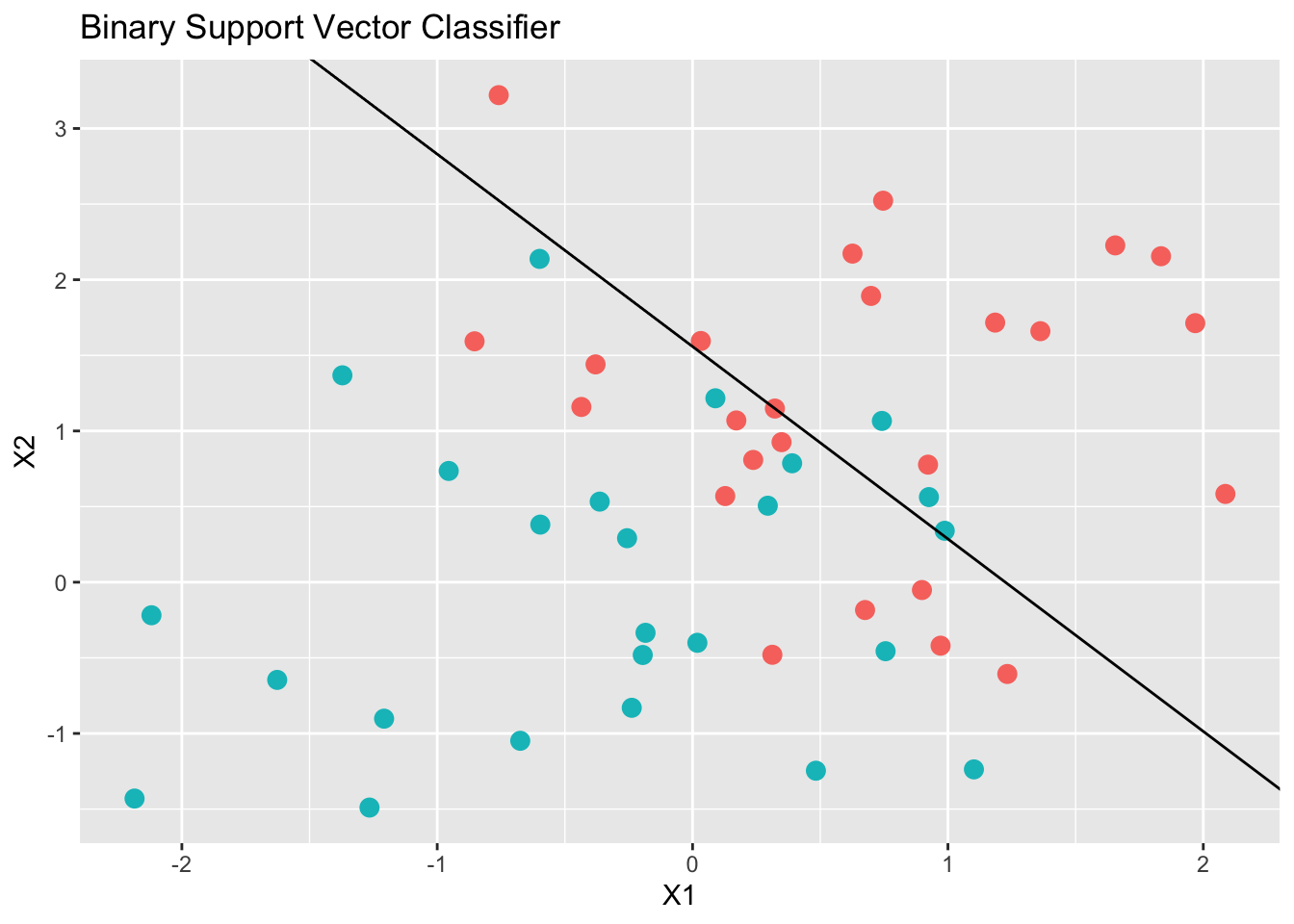
Disciplined Convex Programming (DCP)
Disciplined convex programming (DCP) is a system for constructing
mathematical expressions with known sign and curvature from a given library of
base functions. CVXR uses DCP to ensure that the specified
optimization problems are convex.
The user may find it helpful to read about how the DCP rules are applied in other languages such as Python, Matlab, and Julia.
CVXR implements the same rules, and a short introduction
is available here. The set of DCP functions are
described in Function Reference.
Session Info
sessionInfo()## R version 4.2.1 (2022-06-23)
## Platform: x86_64-apple-darwin21.6.0 (64-bit)
## Running under: macOS Ventura 13.0
##
## Matrix products: default
## BLAS: /usr/local/Cellar/openblas/0.3.21/lib/libopenblasp-r0.3.21.dylib
## LAPACK: /usr/local/Cellar/r/4.2.1_4/lib/R/lib/libRlapack.dylib
##
## locale:
## [1] en_US.UTF-8/en_US.UTF-8/en_US.UTF-8/C/en_US.UTF-8/en_US.UTF-8
##
## attached base packages:
## [1] stats graphics grDevices datasets utils methods base
##
## other attached packages:
## [1] MASS_7.3-58.1 tidyr_1.2.1 ggplot2_3.3.6 CVXR_1.0-11
##
## loaded via a namespace (and not attached):
## [1] tidyselect_1.2.0 xfun_0.34 bslib_0.4.0 slam_0.1-50
## [5] purrr_0.3.5 lattice_0.20-45 Rmosek_10.0.25 colorspace_2.0-3
## [9] vctrs_0.5.0 generics_0.1.3 htmltools_0.5.3 yaml_2.3.6
## [13] gmp_0.6-6 utf8_1.2.2 rlang_1.0.6 jquerylib_0.1.4
## [17] pillar_1.8.1 glue_1.6.2 Rmpfr_0.8-9 withr_2.5.0
## [21] DBI_1.1.3 Rcplex_0.3-5 bit64_4.0.5 lifecycle_1.0.3
## [25] stringr_1.4.1 munsell_0.5.0 blogdown_1.13 gtable_0.3.1
## [29] gurobi_9.5-2 codetools_0.2-18 evaluate_0.17 labeling_0.4.2
## [33] knitr_1.40 fastmap_1.1.0 cccp_0.2-9 fansi_1.0.3
## [37] highr_0.9 Rcpp_1.0.9 scales_1.2.1 cachem_1.0.6
## [41] osqp_0.6.0.5 jsonlite_1.8.3 farver_2.1.1 bit_4.0.4
## [45] digest_0.6.30 stringi_1.7.8 bookdown_0.29 dplyr_1.0.10
## [49] Rglpk_0.6-4 grid_4.2.1 cli_3.4.1 tools_4.2.1
## [53] magrittr_2.0.3 sass_0.4.2 tibble_3.1.8 pkgconfig_2.0.3
## [57] ellipsis_0.3.2 rcbc_0.1.0.9001 Matrix_1.5-1 assertthat_0.2.1
## [61] rmarkdown_2.17 R6_2.5.1 compiler_4.2.1