Direct Standardization
Introduction
Consider a set of observations \((x_i,y_i)\) drawn non-uniformly from an unknown distribution. We know the expected value of the columns of \(X\), denoted by \(b \in {\mathbf R}^n\), and want to estimate the true distribution of \(y\). This situation may arise, for instance, if we wish to analyze the health of a population based on a sample skewed toward young males, knowing the average population-level sex, age, etc. The empirical distribution that places equal probability \(1/m\) on each \(y_i\) is not a good estimate.
So, we must determine the weights \(w \in {\mathbf R}^m\) of a weighted empirical distribution, \(y = y_i\) with probability \(w_i\), which rectifies the skewness of the sample (Fleiss, Levin, and Paik 2003, 19.5). We can pose this problem as
\[ \begin{array}{ll} \underset{w}{\mbox{maximize}} & \sum_{i=1}^m -w_i\log w_i \\ \mbox{subject to} & w \geq 0, \quad \sum_{i=1}^m w_i = 1,\quad X^Tw = b. \end{array} \]
Our objective is the total entropy, which is concave on \({\mathbf R}_+^m\), and our constraints ensure \(w\) is a probability distribution that implies our known expectations on \(X\).
To illustrate this method, we generate \(m = 1000\) data points \(x_{i,1} \sim \mbox{Bernoulli}(0.5)\), \(x_{i,2} \sim \mbox{Uniform}(10,60)\), and \(y_i \sim N(5x_{i,1} + 0.1x_{i,2},1)\). Then we construct a skewed sample of \(m = 100\) points that overrepresent small values of \(y_i\), thus biasing its distribution downwards. This can be seen in Figure \(\ref{fig:direct-std}\), where the sample probability distribution peaks around \(y = 2.0\), and its cumulative distribution is shifted left from the population’s curve. Using direct standardization, we estimate \(w_i\) and reweight our sample; the new empirical distribution cleaves much closer to the true distribution shown in red.
In the CVXR code below, we import data from the package and solve
for \(w\).
## Import problem data
data(dspop)   # Population
data(dssamp)  # Skewed sample

ypop <- dspop[,1]
Xpop <- dspop[,-1]
y <- dssamp[,1]
X <- dssamp[,-1]
m <- nrow(X)

## Given population mean of features
b <- as.matrix(apply(Xpop, 2, mean))

## Construct the direct standardization problem
w <- Variable(m)
objective <- sum(entr(w))
constraints <- list(w >= 0, sum(w) == 1, t(X) %*% w == b)
prob <- Problem(Maximize(objective), constraints)

## Solve for the distribution weights
result <- solve(prob)
weights <- result$getValue(w)
result$value
## [1] 4.223305We can plot the density functions using linear approximations for the range of \(y\).
## Plot probability density functions
dens1 <- density(ypop)
dens2 <- density(y)
dens3 <- density(y, weights = weights)
## Warning in density.default(y, weights = weights): Selecting bandwidth *not*
## using 'weights'yrange <- seq(-3, 15, 0.01)
d <- data.frame(x = yrange,
True = approx(x = dens1$x, y = dens1$y, xout = yrange)$y,
Sample = approx(x = dens2$x, y = dens2$y, xout = yrange)$y,
Weighted = approx(x = dens3$x, y = dens3$y, xout = yrange)$y)
plot.data <- gather(data = d, key = "Type", value = "Estimate", True, Sample, Weighted,
factor_key = TRUE)
ggplot(plot.data) +
geom_line(mapping = aes(x = x, y = Estimate, color = Type)) +
theme(legend.position = "top")## Warning: Removed 300 rows containing missing values or values outside the scale
## range (`geom_line()`).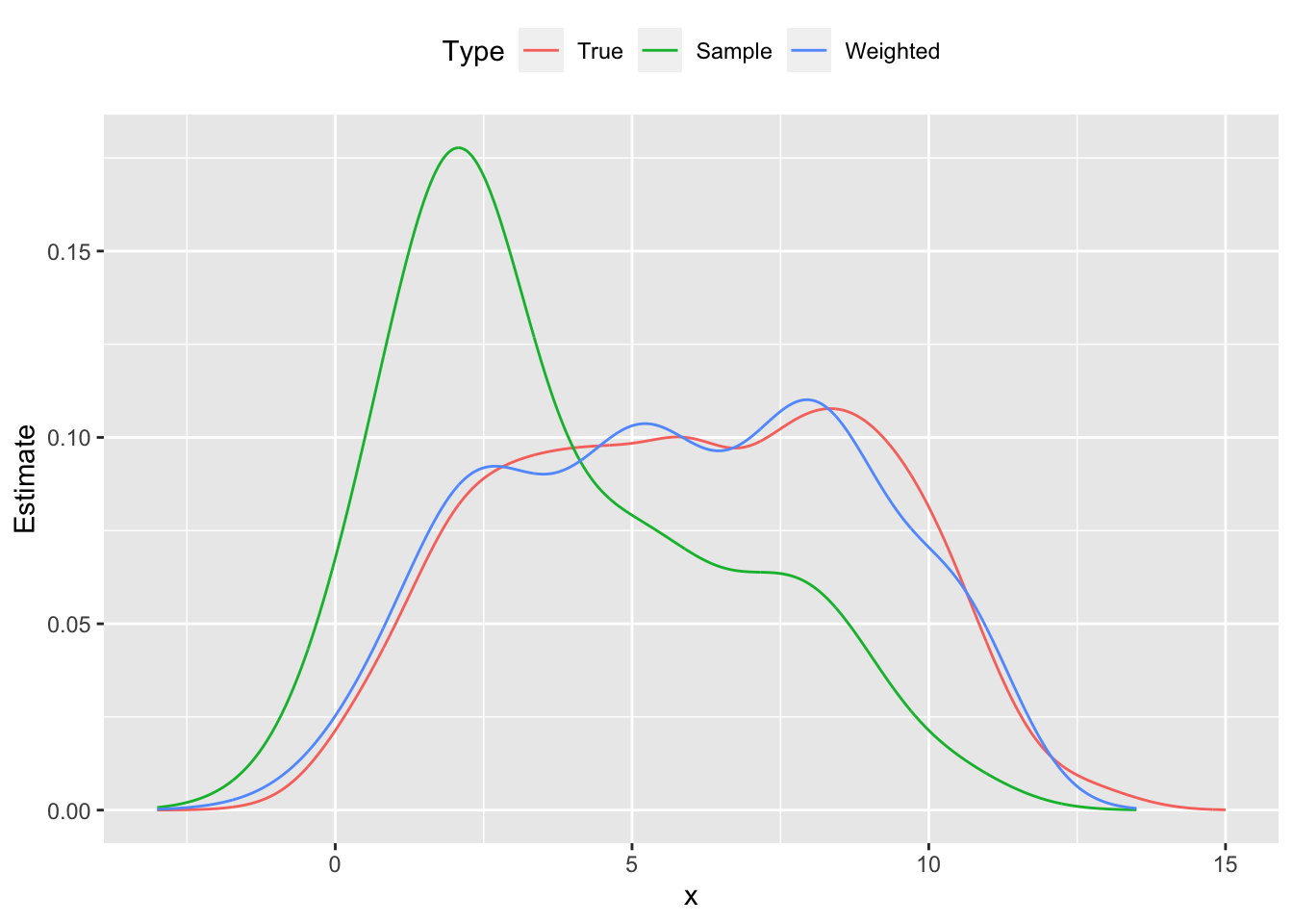
Figure 1: Probability distribution functions population, skewed sample and reweighted sample
Followed by the cumulative distribution function.
## Return the cumulative distribution function
get_cdf <- function(data, probs, color = 'k') {
    if(missing(probs))
        probs <- rep(1.0/length(data), length(data))
    distro <- cbind(data, probs)
    dsort <- distro[order(distro[,1]),]
    ecdf <- base::cumsum(dsort[,2])
    cbind(dsort[,1], ecdf)
}

## Plot cumulative distribution functions
d1 <- data.frame("True", get_cdf(ypop))
d2 <- data.frame("Sample", get_cdf(y))
d3 <- data.frame("Weighted", get_cdf(y, weights))

names(d1) <- names(d2) <- names(d3) <- c("Type", "x", "Estimate")
plot.data <- rbind(d1, d2, d3)

ggplot(plot.data) +
    geom_line(mapping = aes(x = x, y = Estimate, color = Type)) +
    theme(legend.position = "top")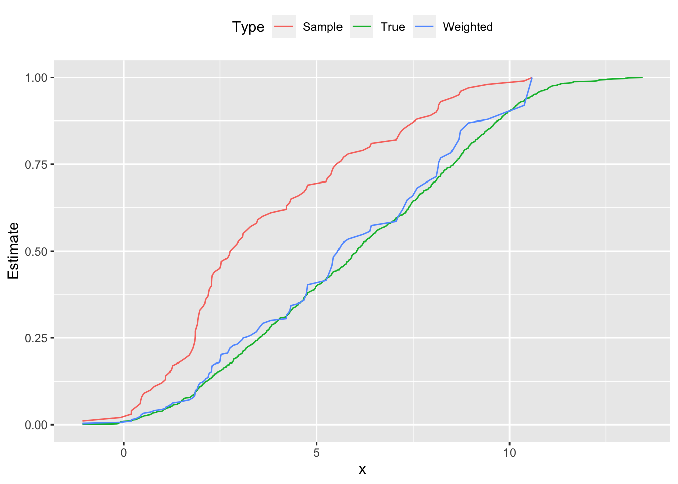
## Testthat Results: No output is goodSession Info
sessionInfo()## R version 4.4.1 (2024-06-14)
## Platform: x86_64-apple-darwin20
## Running under: macOS Sonoma 14.5
##
## Matrix products: default
## BLAS: /Library/Frameworks/R.framework/Versions/4.4-x86_64/Resources/lib/libRblas.0.dylib
## LAPACK: /Library/Frameworks/R.framework/Versions/4.4-x86_64/Resources/lib/libRlapack.dylib; LAPACK version 3.12.0
##
## locale:
## [1] en_US.UTF-8/en_US.UTF-8/en_US.UTF-8/C/en_US.UTF-8/en_US.UTF-8
##
## time zone: America/Los_Angeles
## tzcode source: internal
##
## attached base packages:
## [1] stats graphics grDevices datasets utils methods base
##
## other attached packages:
## [1] tidyr_1.3.1 ggplot2_3.5.1 CVXR_1.0-15 testthat_3.2.1.1
## [5] here_1.0.1
##
## loaded via a namespace (and not attached):
## [1] gmp_0.7-4 clarabel_0.9.0 sass_0.4.9 utf8_1.2.4
## [5] generics_0.1.3 slam_0.1-50 blogdown_1.19 lattice_0.22-6
## [9] digest_0.6.36 magrittr_2.0.3 evaluate_0.24.0 grid_4.4.1
## [13] bookdown_0.40 pkgload_1.4.0 fastmap_1.2.0 rprojroot_2.0.4
## [17] jsonlite_1.8.8 Matrix_1.7-0 ECOSolveR_0.5.5 brio_1.1.5
## [21] Rmosek_10.2.0 purrr_1.0.2 fansi_1.0.6 scales_1.3.0
## [25] codetools_0.2-20 jquerylib_0.1.4 cli_3.6.3 Rmpfr_0.9-5
## [29] rlang_1.1.4 Rglpk_0.6-5.1 bit64_4.0.5 munsell_0.5.1
## [33] withr_3.0.0 cachem_1.1.0 yaml_2.3.9 tools_4.4.1
## [37] Rcplex_0.3-6 rcbc_0.1.0.9001 dplyr_1.1.4 colorspace_2.1-0
## [41] gurobi_11.0-0 assertthat_0.2.1 vctrs_0.6.5 R6_2.5.1
## [45] lifecycle_1.0.4 bit_4.0.5 desc_1.4.3 cccp_0.3-1
## [49] pkgconfig_2.0.3 bslib_0.7.0 pillar_1.9.0 gtable_0.3.5
## [53] glue_1.7.0 Rcpp_1.0.12 highr_0.11 xfun_0.45
## [57] tibble_3.2.1 tidyselect_1.2.1 knitr_1.48 farver_2.1.2
## [61] htmltools_0.5.8.1 labeling_0.4.3 rmarkdown_2.27 compiler_4.4.1