Quantile Regression

Introduction

Quantile regression is another variation on least squares . The loss is the tilted \(l_1\) function,

\[ \phi(u) = \tau\max(u,0) - (1-\tau)\max(-u,0) = \frac{1}{2}|u| + \left(\tau - \frac{1}{2}\right)u, \]

where \(\tau \in (0,1)\) specifies the quantile. The problem as before is to minimize the total residual loss. This model is commonly used in ecology, healthcare, and other fields where the mean alone is not enough to capture complex relationships between variables. CVXR allows us to create a function to represent the loss and integrate it seamlessly into the problem definition, as illustrated below.

Example

We will use an example from the quantreg package. The vignette provides an example of the estimation and plot.

data(engel)
p <- ggplot(data = engel) +
    geom_point(mapping = aes(x = income, y = foodexp), color = "blue")
taus <- c(0.1, 0.25, 0.5, 0.75, 0.90, 0.95)
fits <- data.frame(
    coef(lm(foodexp ~ income, data = engel)),
    sapply(taus, function(x) coef(rq(formula = foodexp ~ income, data = engel, tau = x))))
names(fits) <- c("OLS", sprintf("$\\tau_{%0.2f}$", taus))

nf <- ncol(fits)
colors <- colorRampPalette(colors = c("black", "red"))(nf)
p <- p + geom_abline(intercept = fits[1, 1], slope = fits[2, 1], color = colors[1], size = 1.5)
for (i in seq_len(nf)[-1]) {
    p <- p + geom_abline(intercept = fits[1, i], slope = fits[2, i], color = colors[i])
}
p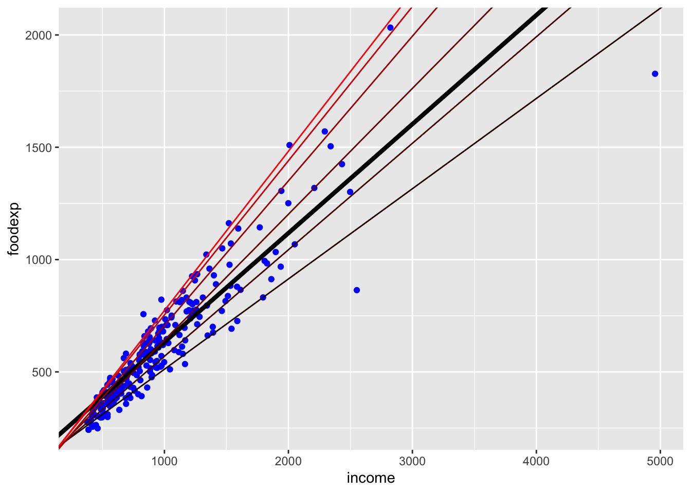

The above plot shows the quantile regression fits for \(\tau = (0.1, 0.25, 0.5, 0.75, 0.90, 0.95)\). The OLS fit is the thick black line.

The following is a table of the estimates.

knitr::kable(fits, format = "html", caption = "Fits from OLS and `quantreg`") %>%
    kable_styling("striped") %>%
    column_spec(1:8, background = "#ececec")

The CVXR formulation follows. Note we make use of model.matrix to get the intercept column painlessly.

X <- model.matrix(foodexp ~ income, data = engel)
y <- matrix(engel[, "foodexp"], ncol = 1)
beta <- Variable(2)
quant_loss <- function(u, tau) { 0.5 * abs(u) + (tau - 0.5) * u }
solutions <- sapply(taus, function(tau) {
    obj <- sum(quant_loss(y - X %*% beta, t = tau))
    prob <- Problem(Minimize(obj))
    ## THE OSQP solver returns an error for tau = 0.5
    solve(prob, solver = "ECOS")$getValue(beta)
})
fits <- data.frame(coef(lm(foodexp ~ income, data = engel)),
                   solutions)
names(fits) <- c("OLS", sprintf("$\\tau_{%0.2f}$", taus))

Here is a table similar to the above with the OLS estimate added in for easy comparison.

knitr::kable(fits, format = "html", caption = "Fits from OLS and `CVXR`") %>%
    kable_styling("striped") %>%
    column_spec(1:8, background = "#ececec")

The results match.

Session Info

sessionInfo()

## R version 4.2.1 (2022-06-23)
## Platform: x86_64-apple-darwin21.6.0 (64-bit)
## Running under: macOS Ventura 13.0
## 
## Matrix products: default
## BLAS:   /usr/local/Cellar/openblas/0.3.21/lib/libopenblasp-r0.3.21.dylib
## LAPACK: /usr/local/Cellar/r/4.2.1_4/lib/R/lib/libRlapack.dylib
## 
## locale:
## [1] en_US.UTF-8/en_US.UTF-8/en_US.UTF-8/C/en_US.UTF-8/en_US.UTF-8
## 
## attached base packages:
## [1] stats     graphics  grDevices datasets  utils     methods   base     
## 
## other attached packages:
## [1] quantreg_5.94    SparseM_1.81     kableExtra_1.3.4 ggplot2_3.3.6   
## [5] CVXR_1.0-11     
## 
## loaded via a namespace (and not attached):
##  [1] Rcpp_1.0.9         gurobi_9.5-2       svglite_2.1.0      lattice_0.20-45   
##  [5] Rmosek_10.0.25     rcbc_0.1.0.9001    assertthat_0.2.1   digest_0.6.30     
##  [9] utf8_1.2.2         gmp_0.6-6          slam_0.1-50        R6_2.5.1          
## [13] MatrixModels_0.5-1 evaluate_0.17      httr_1.4.4         highr_0.9         
## [17] blogdown_1.13      pillar_1.8.1       rlang_1.0.6        rstudioapi_0.14   
## [21] jquerylib_0.1.4    Matrix_1.5-1       rmarkdown_2.17     labeling_0.4.2    
## [25] splines_4.2.1      webshot_0.5.4      stringr_1.4.1      bit_4.0.4         
## [29] munsell_0.5.0      compiler_4.2.1     xfun_0.34          pkgconfig_2.0.3   
## [33] systemfonts_1.0.4  Rglpk_0.6-4        htmltools_0.5.3    Rcplex_0.3-5      
## [37] tidyselect_1.2.0   tibble_3.1.8       bookdown_0.29      codetools_0.2-18  
## [41] fansi_1.0.3        viridisLite_0.4.1  dplyr_1.0.10       withr_2.5.0       
## [45] MASS_7.3-58.1      grid_4.2.1         jsonlite_1.8.3     gtable_0.3.1      
## [49] lifecycle_1.0.3    DBI_1.1.3          magrittr_2.0.3     scales_1.2.1      
## [53] cli_3.4.1          stringi_1.7.8      cachem_1.0.6       farver_2.1.1      
## [57] Rmpfr_0.8-9        xml2_1.3.3         bslib_0.4.0        generics_0.1.3    
## [61] vctrs_0.5.0        tools_4.2.1        bit64_4.0.5        glue_1.6.2        
## [65] fastmap_1.1.0      survival_3.4-0     yaml_2.3.6         colorspace_2.0-3  
## [69] cccp_0.2-9         rvest_1.0.3        ECOSolveR_0.5.4    knitr_1.40        
## [73] sass_0.4.2

Source

R Markdown

References