Elastic Net
Introduction
Often in applications, we encounter problems that require regularization to prevent overfitting, introduce sparsity, facilitate variable selection, or impose prior distributions on parameters. Two of the most common regularization functions are the \(l_1\)-norm and squared \(l_2\)-norm, combined in the elastic net regression model Friedman, Hastie, and Tibshirani (2010),
\[ \begin{array}{ll} \underset{\beta}{\mbox{minimize}} & \frac{1}{2m}\|y - X\beta\|_2^2 + \lambda(\frac{1-\alpha}{2}\|\beta\|_2^2 + \alpha\|\beta\|_1). \end{array} \]
Here \(\lambda \geq 0\) is the overall regularization weight and \(\alpha \in [0,1]\) controls the relative \(l_1\) versus squared \(l_2\) penalty. Thus, this model encompasses both ridge (\(\alpha = 0\)) and lasso (\(\alpha = 1\)) regression.
Example
To solve this problem in CVXR, we first define a function that
calculates the regularization term given the variable and penalty
weights.
elastic_reg <- function(beta, lambda = 0, alpha = 0) {
    ridge <- (1 - alpha) / 2 * sum(beta^2)
    lasso <- alpha * p_norm(beta, 1)
    lambda * (lasso + ridge)
}
Later, we will add it to the scaled least squares loss as shown below.
loss <- sum((y - X %*% beta)^2) / (2 * n)
obj <- loss + elastic_reg(beta, lambda, alpha)
The advantage of this modular approach is that we can easily
incorporate elastic net regularization into other regression
models. For instance, if we wanted to run regularized Huber
regression, CVXR allows us to reuse the above code with just a
single changed line.
loss <- huber(y - X %*% beta, M)We generate some synthetic sparse data for this example.
set.seed(1)

# Problem data
p <- 20
n <- 1000
DENSITY <- 0.25    # Fraction of non-zero beta
beta_true <- matrix(rnorm(p), ncol = 1)
idxs <- sample.int(p, size = floor((1 - DENSITY) * p), replace = FALSE)
beta_true[idxs] <- 0

sigma <- 45
X <- matrix(rnorm(n * p, sd = 5), nrow = n, ncol = p)
eps <- matrix(rnorm(n, sd = sigma), ncol = 1)
y <- X %*% beta_true + eps
We fit the elastic net model for several values of \(\lambda\) .
TRIALS <- 10
beta_vals <- matrix(0, nrow = p, ncol = TRIALS)
lambda_vals <- 10^seq(-2, log10(50), length.out = TRIALS)
beta <- Variable(p)
loss <- sum((y - X %*% beta)^2) / (2 * n)

## Elastic-net regression
alpha <- 0.75
beta_vals <- sapply(lambda_vals,
                    function (lambda) {
                        obj <- loss + elastic_reg(beta, lambda, alpha)
                        prob <- Problem(Minimize(obj))
                        result <- solve(prob)
                        result$getValue(beta)
                    })
We can now get a table of the coefficients.
d <- as.data.frame(beta_vals)
rownames(d) <- sprintf("$\\beta_{%d}$", seq_len(p))
names(d) <- sprintf("$\\lambda = %.3f$", lambda_vals)
knitr::kable(d, format = "html", caption = "Elastic net fits from `CVXR`", digits = 3) %>%
    kable_styling("striped") %>%
column_spec(1:11, background = "#ececec")| \(\lambda = 0.010\) | \(\lambda = 0.026\) | \(\lambda = 0.066\) | \(\lambda = 0.171\) | \(\lambda = 0.441\) | \(\lambda = 1.135\) | \(\lambda = 2.924\) | \(\lambda = 7.533\) | \(\lambda = 19.408\) | \(\lambda = 50.000\) | |
|---|---|---|---|---|---|---|---|---|---|---|
| \(\beta_{1}\) | 0.002 | 0.002 | 0.001 | 0.000 | 0.000 | 0.000 | 0.000 | 0.000 | 0.000 | 0.000 |
| \(\beta_{2}\) | -0.035 | -0.035 | -0.033 | -0.030 | -0.022 | 0.000 | 0.000 | 0.000 | 0.000 | 0.000 |
| \(\beta_{3}\) | 0.379 | 0.378 | 0.376 | 0.372 | 0.362 | 0.334 | 0.267 | 0.101 | 0.000 | 0.000 |
| \(\beta_{4}\) | 1.812 | 1.811 | 1.809 | 1.804 | 1.790 | 1.755 | 1.666 | 1.453 | 0.983 | 0.135 |
| \(\beta_{5}\) | -0.410 | -0.409 | -0.408 | -0.404 | -0.395 | -0.371 | -0.310 | -0.169 | 0.000 | 0.000 |
| \(\beta_{6}\) | 0.352 | 0.352 | 0.350 | 0.346 | 0.336 | 0.309 | 0.245 | 0.082 | 0.000 | 0.000 |
| \(\beta_{7}\) | 0.397 | 0.397 | 0.395 | 0.392 | 0.382 | 0.358 | 0.297 | 0.152 | 0.000 | 0.000 |
| \(\beta_{8}\) | 0.098 | 0.098 | 0.096 | 0.093 | 0.085 | 0.064 | 0.011 | 0.000 | 0.000 | 0.000 |
| \(\beta_{9}\) | -0.051 | -0.051 | -0.049 | -0.046 | -0.039 | -0.020 | 0.000 | 0.000 | 0.000 | 0.000 |
| \(\beta_{10}\) | 0.084 | 0.083 | 0.082 | 0.079 | 0.071 | 0.051 | 0.001 | 0.000 | 0.000 | 0.000 |
| \(\beta_{11}\) | 1.134 | 1.133 | 1.132 | 1.128 | 1.117 | 1.090 | 1.020 | 0.853 | 0.494 | 0.000 |
| \(\beta_{12}\) | 0.092 | 0.092 | 0.091 | 0.089 | 0.082 | 0.066 | 0.024 | 0.000 | 0.000 | 0.000 |
| \(\beta_{13}\) | -0.428 | -0.427 | -0.425 | -0.420 | -0.408 | -0.378 | -0.301 | -0.112 | 0.000 | 0.000 |
| \(\beta_{14}\) | -0.113 | -0.112 | -0.111 | -0.107 | -0.096 | -0.070 | -0.003 | 0.000 | 0.000 | 0.000 |
| \(\beta_{15}\) | -0.676 | -0.675 | -0.674 | -0.670 | -0.660 | -0.636 | -0.573 | -0.404 | -0.063 | 0.000 |
| \(\beta_{16}\) | 0.275 | 0.274 | 0.272 | 0.268 | 0.258 | 0.231 | 0.165 | 0.011 | 0.000 | 0.000 |
| \(\beta_{17}\) | -0.004 | -0.004 | -0.003 | 0.000 | 0.000 | 0.000 | 0.000 | 0.000 | 0.000 | 0.000 |
| \(\beta_{18}\) | 0.186 | 0.185 | 0.184 | 0.180 | 0.170 | 0.144 | 0.082 | 0.000 | 0.000 | 0.000 |
| \(\beta_{19}\) | -0.517 | -0.516 | -0.514 | -0.509 | -0.497 | -0.465 | -0.387 | -0.210 | 0.000 | 0.000 |
| \(\beta_{20}\) | 0.761 | 0.761 | 0.759 | 0.755 | 0.745 | 0.719 | 0.656 | 0.487 | 0.109 | 0.000 |
We plot the coefficients against the regularization.
plot(0, 0, type = "n", main = "Regularization Path for Elastic-net Regression",
     xlab = expression(lambda), ylab = expression(beta),
     ylim = c(-0.75, 1.25), xlim = c(0, 50))
matlines(lambda_vals, t(beta_vals))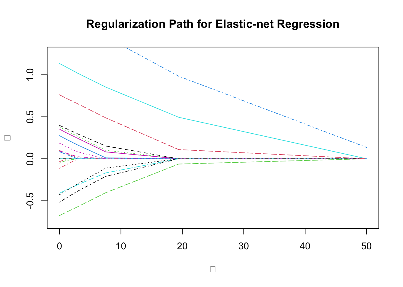
We can also compare with the glmnet results.
model_net <- glmnet(X, y, family = "gaussian", alpha = alpha,
                    lambda = lambda_vals, standardize = FALSE,
                    intercept = FALSE)
## Reverse order to match beta_vals
coef_net <- as.data.frame(as.matrix(coef(model_net)[-1, seq(TRIALS, 1, by = -1)]))
rownames(coef_net) <- sprintf("$\\beta_{%d}$", seq_len(p))
names(coef_net) <- sprintf("$\\lambda = %.3f$", lambda_vals)
knitr::kable(coef_net, format = "html", digits = 3, caption = "Coefficients from `glmnet`") %>%
    kable_styling("striped") %>%
column_spec(1:11, background = "#ececec")| \(\lambda = 0.010\) | \(\lambda = 0.026\) | \(\lambda = 0.066\) | \(\lambda = 0.171\) | \(\lambda = 0.441\) | \(\lambda = 1.135\) | \(\lambda = 2.924\) | \(\lambda = 7.533\) | \(\lambda = 19.408\) | \(\lambda = 50.000\) | |
|---|---|---|---|---|---|---|---|---|---|---|
| \(\beta_{1}\) | 0.002 | 0.002 | 0.001 | 0.000 | 0.000 | 0.000 | 0.000 | 0.000 | 0.000 | 0.000 |
| \(\beta_{2}\) | -0.035 | -0.035 | -0.033 | -0.030 | -0.022 | 0.000 | 0.000 | 0.000 | 0.000 | 0.000 |
| \(\beta_{3}\) | 0.379 | 0.378 | 0.377 | 0.373 | 0.364 | 0.339 | 0.277 | 0.111 | 0.000 | 0.000 |
| \(\beta_{4}\) | 1.812 | 1.812 | 1.811 | 1.807 | 1.798 | 1.776 | 1.717 | 1.568 | 1.183 | 0.205 |
| \(\beta_{5}\) | -0.410 | -0.409 | -0.408 | -0.405 | -0.397 | -0.376 | -0.320 | -0.184 | 0.000 | 0.000 |
| \(\beta_{6}\) | 0.353 | 0.352 | 0.351 | 0.347 | 0.337 | 0.313 | 0.253 | 0.088 | 0.000 | 0.000 |
| \(\beta_{7}\) | 0.398 | 0.397 | 0.396 | 0.392 | 0.384 | 0.361 | 0.304 | 0.158 | 0.000 | 0.000 |
| \(\beta_{8}\) | 0.098 | 0.098 | 0.097 | 0.093 | 0.085 | 0.063 | 0.008 | 0.000 | 0.000 | 0.000 |
| \(\beta_{9}\) | -0.051 | -0.051 | -0.049 | -0.047 | -0.039 | -0.020 | 0.000 | 0.000 | 0.000 | 0.000 |
| \(\beta_{10}\) | 0.084 | 0.083 | 0.082 | 0.079 | 0.071 | 0.051 | 0.001 | 0.000 | 0.000 | 0.000 |
| \(\beta_{11}\) | 1.134 | 1.134 | 1.133 | 1.130 | 1.122 | 1.102 | 1.048 | 0.911 | 0.580 | 0.000 |
| \(\beta_{12}\) | 0.092 | 0.092 | 0.091 | 0.089 | 0.082 | 0.066 | 0.022 | 0.000 | 0.000 | 0.000 |
| \(\beta_{13}\) | -0.428 | -0.427 | -0.426 | -0.422 | -0.411 | -0.384 | -0.315 | -0.130 | 0.000 | 0.000 |
| \(\beta_{14}\) | -0.113 | -0.112 | -0.111 | -0.107 | -0.097 | -0.071 | -0.003 | 0.000 | 0.000 | 0.000 |
| \(\beta_{15}\) | -0.676 | -0.675 | -0.674 | -0.671 | -0.663 | -0.643 | -0.590 | -0.433 | -0.071 | 0.000 |
| \(\beta_{16}\) | 0.275 | 0.274 | 0.273 | 0.269 | 0.259 | 0.234 | 0.171 | 0.014 | 0.000 | 0.000 |
| \(\beta_{17}\) | -0.004 | -0.004 | -0.003 | 0.000 | 0.000 | 0.000 | 0.000 | 0.000 | 0.000 | 0.000 |
| \(\beta_{18}\) | 0.186 | 0.185 | 0.184 | 0.180 | 0.170 | 0.145 | 0.085 | 0.000 | 0.000 | 0.000 |
| \(\beta_{19}\) | -0.517 | -0.516 | -0.514 | -0.510 | -0.499 | -0.472 | -0.400 | -0.226 | 0.000 | 0.000 |
| \(\beta_{20}\) | 0.761 | 0.761 | 0.760 | 0.756 | 0.748 | 0.728 | 0.678 | 0.529 | 0.137 | 0.000 |
## Testthat Results: No output is good## Error: `beta_vals` not identical to e_net$beta_vals.
## 7/200 mismatches (average diff: 8.83e-08)
## [41] 0.001150 - 0.001150 == -1.00e-07
## [61] 0.000222 - 0.000222 == -1.50e-07
## [71] 1.127833 - 1.127833 == 1.63e-08
## [72] 0.088552 - 0.088552 == 2.15e-08
## [74] -0.106758 - -0.106758 == -1.76e-08
## [77] -0.000382 - -0.000382 == 2.65e-07
## [102] -0.000237 - -0.000237 == 4.74e-08Session Info
sessionInfo()## R version 4.4.1 (2024-06-14)
## Platform: x86_64-apple-darwin20
## Running under: macOS Sonoma 14.5
##
## Matrix products: default
## BLAS: /Library/Frameworks/R.framework/Versions/4.4-x86_64/Resources/lib/libRblas.0.dylib
## LAPACK: /Library/Frameworks/R.framework/Versions/4.4-x86_64/Resources/lib/libRlapack.dylib; LAPACK version 3.12.0
##
## locale:
## [1] en_US.UTF-8/en_US.UTF-8/en_US.UTF-8/C/en_US.UTF-8/en_US.UTF-8
##
## time zone: America/Los_Angeles
## tzcode source: internal
##
## attached base packages:
## [1] stats graphics grDevices datasets utils methods base
##
## other attached packages:
## [1] glmnet_4.1-8 Matrix_1.7-0 kableExtra_1.4.0 ggplot2_3.5.1
## [5] CVXR_1.0-15 testthat_3.2.1.1 here_1.0.1
##
## loaded via a namespace (and not attached):
## [1] gtable_0.3.5 shape_1.4.6.1 xfun_0.45 bslib_0.7.0
## [5] lattice_0.22-6 Rmosek_10.2.0 vctrs_0.6.5 tools_4.4.1
## [9] generics_0.1.3 tibble_3.2.1 fansi_1.0.6 highr_0.11
## [13] pkgconfig_2.0.3 desc_1.4.3 assertthat_0.2.1 lifecycle_1.0.4
## [17] compiler_4.4.1 stringr_1.5.1 brio_1.1.5 munsell_0.5.1
## [21] gurobi_11.0-0 codetools_0.2-20 htmltools_0.5.8.1 sass_0.4.9
## [25] cccp_0.3-1 yaml_2.3.9 gmp_0.7-4 pillar_1.9.0
## [29] jquerylib_0.1.4 rcbc_0.1.0.9001 clarabel_0.9.0 Rcplex_0.3-6
## [33] cachem_1.1.0 iterators_1.0.14 foreach_1.5.2 tidyselect_1.2.1
## [37] digest_0.6.36 stringi_1.8.4 slam_0.1-50 dplyr_1.1.4
## [41] bookdown_0.40 splines_4.4.1 rprojroot_2.0.4 fastmap_1.2.0
## [45] grid_4.4.1 colorspace_2.1-0 cli_3.6.3 magrittr_2.0.3
## [49] survival_3.7-0 utf8_1.2.4 withr_3.0.0 Rmpfr_0.9-5
## [53] scales_1.3.0 bit64_4.0.5 rmarkdown_2.27 bit_4.0.5
## [57] blogdown_1.19 evaluate_0.24.0 knitr_1.48 Rglpk_0.6-5.1
## [61] viridisLite_0.4.2 rlang_1.1.4 Rcpp_1.0.12 glue_1.7.0
## [65] xml2_1.3.6 pkgload_1.4.0 osqp_0.6.3.3 svglite_2.1.3
## [69] rstudioapi_0.16.0 jsonlite_1.8.8 R6_2.5.1 systemfonts_1.1.0