Fastest Mixing Markov Chain

Introduction

This example is derived from the results in Boyd, Diaconis, and Xiao (2004), section 2. Let \(\mathcal{G} = (\mathcal{V}, \mathcal{E})\) be a connected graph with vertices \(\mathcal{V} = \{1,\ldots,n\}\) and edges \(\mathcal{E} \subseteq \mathcal{V} \times \mathcal{V}\). Assume that \((i,i) \in \mathcal{E}\) for all \(i = 1,\ldots,n\), and \((i,j) \in \mathcal{E}\) implies \((j,i) \in \mathcal{E}\). Under these conditions, a discrete-time Markov chain on \(\mathcal{V}\) will have the uniform distribution as one of its equilibrium distributions. We are interested in finding the Markov chain, constructing the transition probability matrix \(P \in {\mathbf R}_+^{n \times n}\), that minimizes its asymptotic convergence rate to the uniform distribution. This is an important problem in Markov chain Monte Carlo (MCMC) simulations, as it directly affects the sampling efficiency of an algorithm.

The asymptotic rate of convergence is determined by the second largest eigenvalue of \(P\), which in our case is \(\mu(P) := \lambda_{\max}(P - \frac{1}{n}{\mathbf 1}{\mathbf 1}^T)\) where \(\lambda_{\max}(A)\) denotes the maximum eigenvalue of \(A\). As \(\mu(P)\) decreases, the mixing rate increases and the Markov chain converges faster to equilibrium. Thus, our optimization problem is

\[ \begin{array}{ll} \underset{P}{\mbox{minimize}} & \lambda_{\max}(P - \frac{1}{n}{\mathbf 1}{\mathbf 1}^T) \\ \mbox{subject to} & P \geq 0, \quad P{\mathbf 1} = {\mathbf 1}, \quad P = P^T \\ & P_{ij} = 0, \quad (i,j) \notin \mathcal{E}. \end{array} \]

The element \(P_{ij}\) of our transition matrix is the probability of moving from state \(i\) to state \(j\). Our assumptions imply that \(P\) is nonnegative, symmetric, and doubly stochastic. The last constraint ensures transitions do not occur between unconnected vertices.

The function \(\lambda_{\max}\) is convex, so this problem is solvable in CVXR. For instance, the code for the Markov chain in Figure 2 below (the triangle plus one edge) is

P <- Variable(n,n)
ones <- matrix(1, nrow = n, ncol = 1)

obj <- Minimize(lambda_max(P - 1/n))
constr1 <- list(P >= 0, P %*% ones == ones, P == t(P))
constr2 <- list(P[1,3] == 0, P[1,4] == 0)
prob <- Problem(obj, c(constr1, constr2))
result <- solve(prob)

where we have set \(n = 4\). We could also have specified \(P{\mathbf 1} = {\mathbf 1}\) with sum_entries(P,1) == 1, which uses the sum_entries atom to represent the row sums.

Example

In order to reproduce some of the examples from Boyd, Diaconis, and Xiao (2004), we create functions to build up the graph, solve the optimization problem and finally display the chain graphically.

## Boyd, Diaconis, and Xiao. SIAM Rev. 46 (2004) pgs. 667-689 at pg. 672
## Form the complementary graph
antiadjacency <- function(g) {
    n <- max(as.numeric(names(g)))   ## Assumes names are integers starting from 1
    a <- lapply(1:n, function(i) c())
    names(a) <- 1:n
    for(x in names(g)) {
        for(y in 1:n) {
            if(!(y %in% g[[x]]))
                a[[x]] <- c(a[[x]], y)
        }
    }
    a
}

## Fastest mixing Markov chain on graph g
FMMC <- function(g, verbose = FALSE) {
    a <- antiadjacency(g)
    n <- length(names(a))
    P <- Variable(n, n)
    o <- rep(1, n)
    objective <- Minimize(norm(P - 1.0/n, "2"))
    constraints <- list(P %*% o == o, t(P) == P, P >= 0)
    for(i in names(a)) {
        for(j in a[[i]]) {  ## (i-j) is a not-edge of g!
            idx <- as.numeric(i)
            if(idx != j)
                constraints <- c(constraints, P[idx,j] == 0)
        }
    }
    prob <- Problem(objective, constraints)
    result <- solve(prob)
    if(verbose)
        cat("Status: ", result$status, ", Optimal Value = ", result$value, ", Solver = ", result$solver)
    list(status = result$status, value = result$value, P = result$getValue(P))
}

disp_result <- function(states, P, tol = 1e-3) {
    if(!("markovchain" %in% rownames(installed.packages()))) {
        rownames(P) <- states
        colnames(P) <- states
        print(P)
    } else {
        P[P < tol] <- 0
        P <- P/apply(P, 1, sum)   ## Normalize so rows sum to exactly 1
        mc <- new("markovchain", states = states, transitionMatrix = P)
        plot(mc)
    }
}

Results

Table 1 from Boyd, Diaconis, and Xiao (2004) is reproduced below.

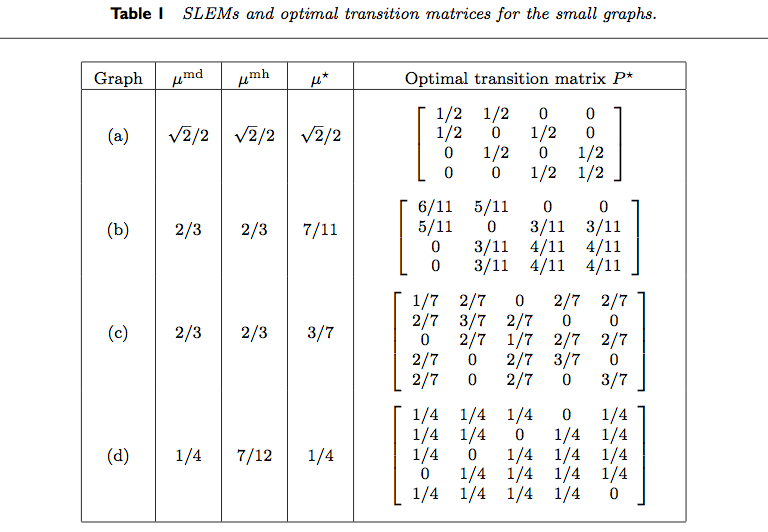
We reproduce the results for various rows of the table.

g <- list("1" = 2, "2" = c(1,3), "3" = c(2,4), "4" = 3)
result1 <- FMMC(g, verbose = TRUE)

## Status:  optimal , Optimal Value =  0.707188 , Solver =  SCS

disp_result(names(g), result1$P)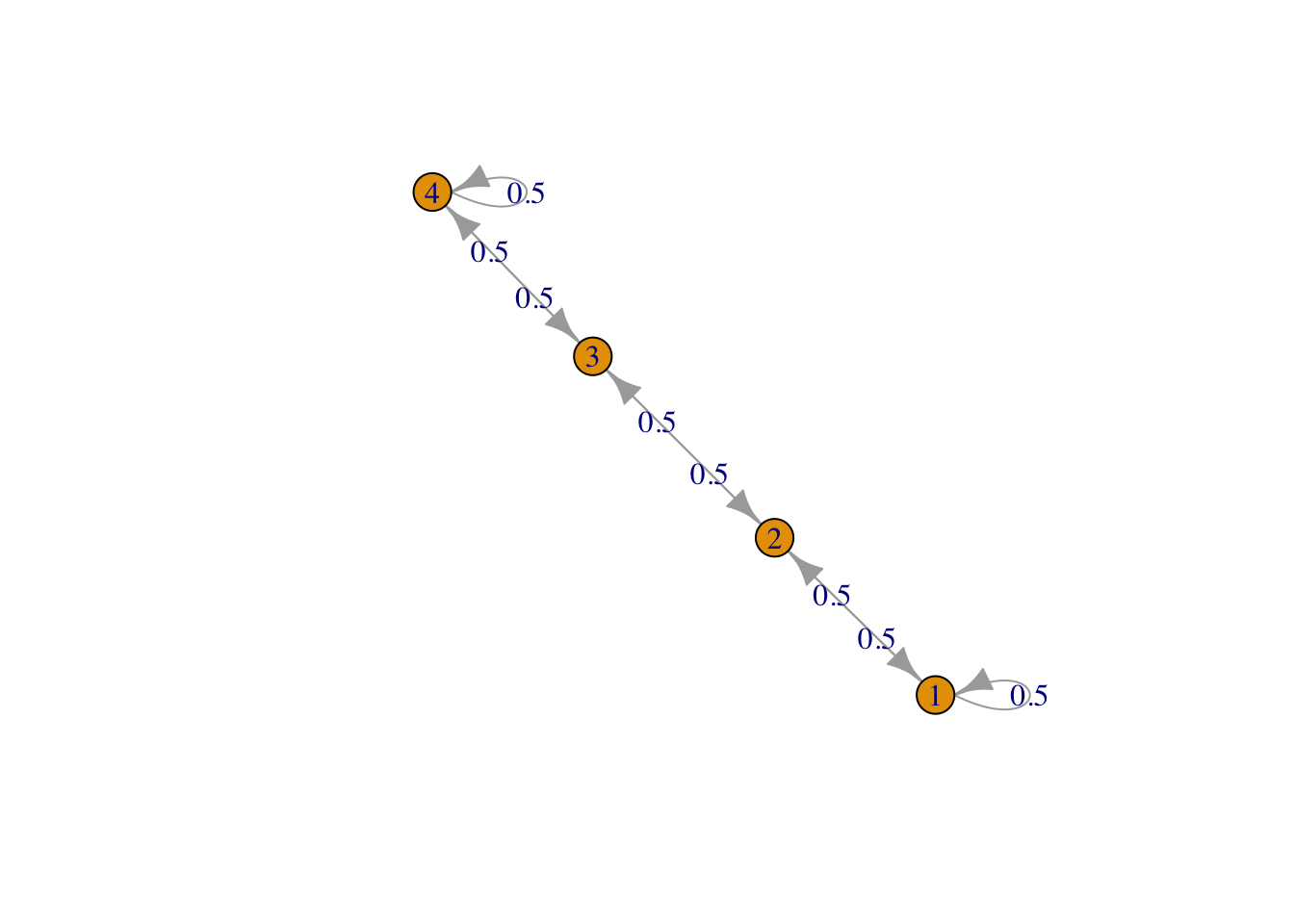

Figure 1: Row 1, line graph

g <- list("1" = 2, "2" = c(1,3,4), "3" = c(2,4), "4" = c(2,3))
result2 <- FMMC(g, verbose = TRUE)

## Status:  optimal , Optimal Value =  0.63641 , Solver =  SCS

disp_result(names(g), result2$P)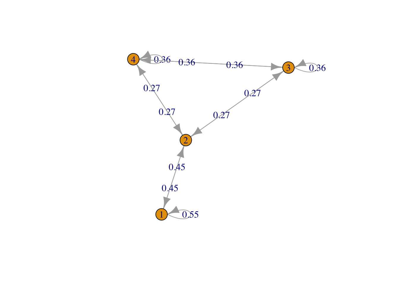

Figure 2: Row 2, triangle plus one edge

g <- list("1" = c(2,4,5), "2" = c(1,3), "3" = c(2,4,5), "4" = c(1,3), "5" = c(1,3))
result3 <- FMMC(g, verbose = TRUE)

## Status:  optimal , Optimal Value =  0.4285398 , Solver =  SCS

disp_result(names(g), result3$P)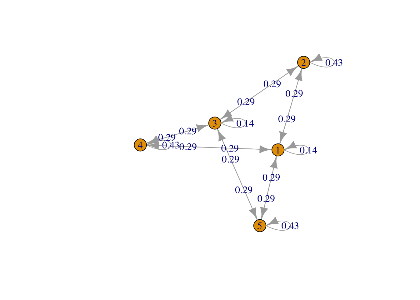

Figure 3: Bipartite 2 plus 3

g <- list("1" = c(2,3,5), "2" = c(1,4,5), "3" = c(1,4,5), "4" = c(2,3,5), "5" = c(1,2,3,4,5))
result4 <- FMMC(g, verbose = TRUE)

## Status:  optimal , Optimal Value =  0.2501638 , Solver =  SCS

disp_result(names(g), result4$P)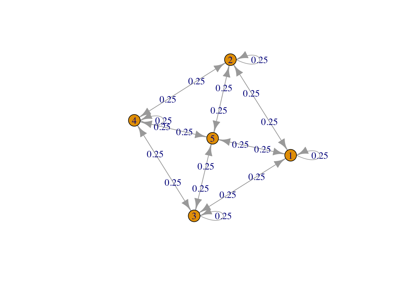

Figure 4: Square plus central point

Extensions

It is easy to extend this example to other Markov chains. To change the number of vertices, we would simply modify n, and to add or remove edges, we need only alter the constraints in constr2. For instance, the bipartite chain in Figure Figure 3 is produced by setting \(n = 5\) and

constr2 <- list(P[1,3] == 0, P[2,4] == 0, P[2,5] == 0, P[4,5] == 0)

Session Info

sessionInfo()

## R version 4.2.1 (2022-06-23)
## Platform: x86_64-apple-darwin21.6.0 (64-bit)
## Running under: macOS Ventura 13.0
## 
## Matrix products: default
## BLAS:   /usr/local/Cellar/openblas/0.3.21/lib/libopenblasp-r0.3.21.dylib
## LAPACK: /usr/local/Cellar/r/4.2.1_4/lib/R/lib/libRlapack.dylib
## 
## locale:
## [1] en_US.UTF-8/en_US.UTF-8/en_US.UTF-8/C/en_US.UTF-8/en_US.UTF-8
## 
## attached base packages:
## [1] stats     graphics  grDevices datasets  utils     methods   base     
## 
## other attached packages:
## [1] markovchain_0.9.0 CVXR_1.0-11      
## 
## loaded via a namespace (and not attached):
##  [1] gmp_0.6-6          Rcpp_1.0.9         highr_0.9          bslib_0.4.0       
##  [5] compiler_4.2.1     jquerylib_0.1.4    tools_4.2.1        digest_0.6.30     
##  [9] bit_4.0.4          jsonlite_1.8.3     evaluate_0.17      lattice_0.20-45   
## [13] pkgconfig_2.0.3    rlang_1.0.6        Matrix_1.5-1       igraph_1.3.5      
## [17] gurobi_9.5-2       cli_3.4.1          Rglpk_0.6-4        yaml_2.3.6        
## [21] parallel_4.2.1     expm_0.999-6       blogdown_1.13      xfun_0.34         
## [25] cccp_0.2-9         fastmap_1.1.0      Rmpfr_0.8-9        stringr_1.4.1     
## [29] knitr_1.40         sass_0.4.2         stats4_4.2.1       bit64_4.0.5       
## [33] grid_4.2.1         R6_2.5.1           rmarkdown_2.17     bookdown_0.29     
## [37] magrittr_2.0.3     scs_3.0-1          codetools_0.2-18   rcbc_0.1.0.9001   
## [41] htmltools_0.5.3    assertthat_0.2.1   Rcplex_0.3-5       stringi_1.7.8     
## [45] Rmosek_10.0.25     RcppParallel_5.1.5 slam_0.1-50        cachem_1.0.6

Source

R Markdown