Log-Concave Distribution Estimation
Introduction
Let n=1 and suppose xi are i.i.d. samples from a log-concave discrete distribution on {0,…,K} for some K∈Z+. Define pk:=Prob(X=k) to be the probability mass function. One method for estimating {p0,…,pK} is to maximize the log-likelihood function subject to a log-concavity constraint , i.e.,
maximizep∑Kk=0Mklogpksubject top≥0,∑Kk=0pk=1,pk≥√pk−1pk+1,k=1,…,K−1,
where p∈RK+1 is our variable of interest and Mk represents the number of observations equal to k, so that ∑Kk=0Mk=m. The problem as posed above is not convex. However, we can transform it into a convex optimization problem by defining new variables uk=logpk and relaxing the equality constraint to ∑Kk=0pk≤1, since the latter always holds tightly at an optimal solution. The result is
maximizeu∑Kk=0Mkuksubject to∑Kk=0euk≤1,uk−uk−1≥uk+1−uk,k=1,…,K−1.
Example
We draw m=25 observations from a log-concave distribution on {0,…,100}. We then estimate the probability mass function using the above method and compare it with the empirical distribution.
set.seed(1)
## Calculate a piecewise linear function
pwl_fun <- function(x, knots) {
    n <- nrow(knots)
    x0 <- sort(knots$x, decreasing = FALSE)
    y0 <- knots$y[order(knots$x, decreasing = FALSE)]
    slope <- diff(y0)/diff(x0)

    sapply(x, function(xs) {
        if(xs <= x0[1])
            y0[1] + slope[1]*(xs -x0[1])
        else if(xs >= x0[n])
            y0[n] + slope[n-1]*(xs - x0[n])
        else {
            idx <- which(xs <= x0)[1]
            y0[idx-1] + slope[idx-1]*(xs - x0[idx-1])
        }
    })
}
## Problem data
m <- 25
xrange <- 0:100
knots <- data.frame(x = c(0, 25, 65, 100), y = c(10, 30, 40, 15))
xprobs <- pwl_fun(xrange, knots)/15
xprobs <- exp(xprobs)/sum(exp(xprobs))
x <- sample(xrange, size = m, replace = TRUE, prob = xprobs)

K <- max(xrange)
counts <- hist(x, breaks = -1:K, right = TRUE, include.lowest = FALSE,
               plot = FALSE)$counts
ggplot() +
geom_histogram(mapping = aes(x = x), breaks = -1:K, color = "blue", fill = "orange")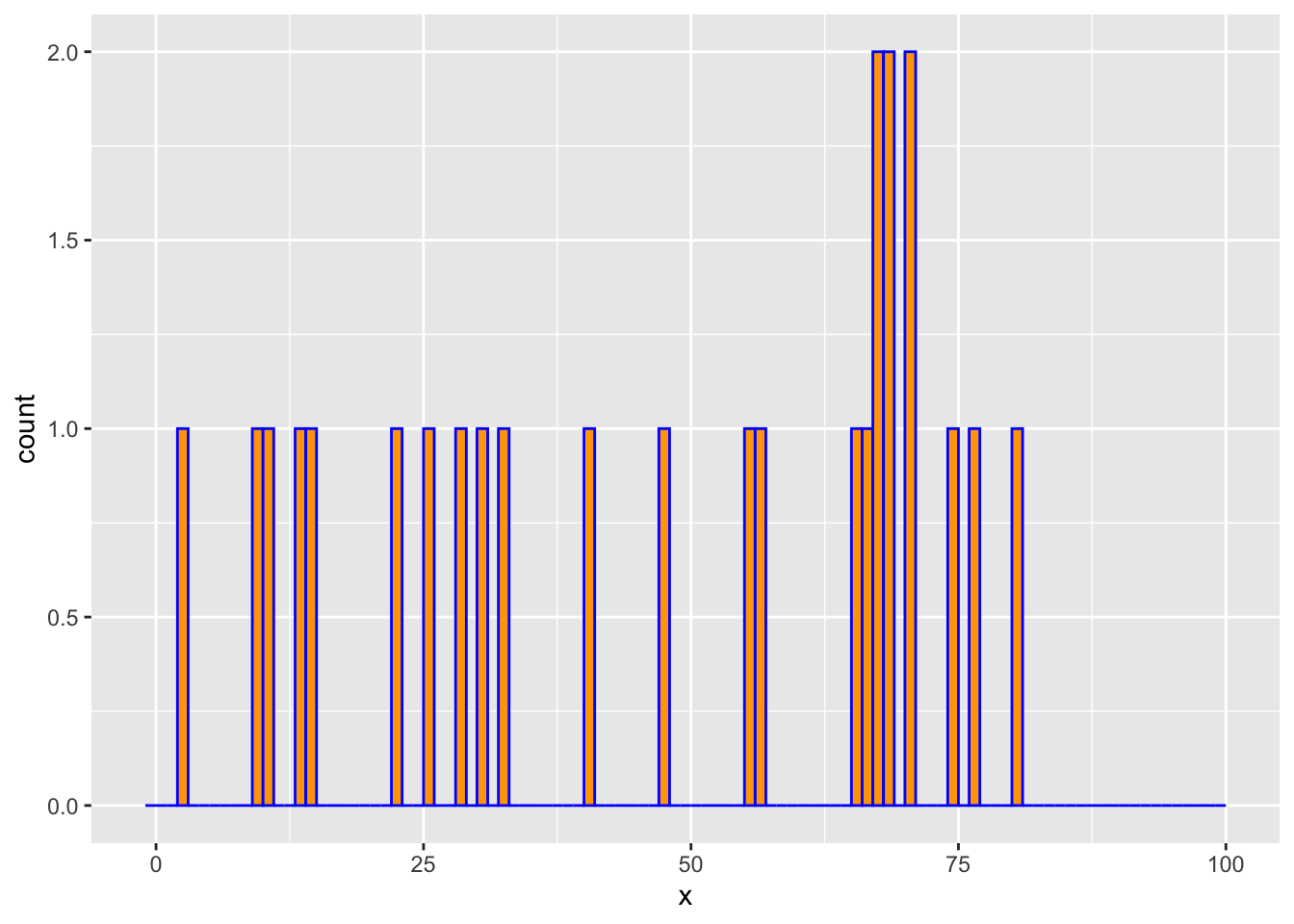
We now solve problem with log-concave constraint.
u <- Variable(K+1)
obj <- t(counts) %*% u
constraints <- list(sum(exp(u)) <= 1, diff(u[1:K]) >= diff(u[2:(K+1)]))
prob <- Problem(Maximize(obj), constraints)
result <- solve(prob)
pmf <- result$getValue(exp(u))
The above lines transform the variables uk to euk before
calculating their resulting values. This is possible because exp is
a member of the CVXR library of atoms, so it can operate directly on
a Variable object such as u.
Below are the comparison plots of pmf and cdf.
dens <- density(x, bw = "sj")
d <- data.frame(x = xrange, True = xprobs, Optimal = pmf,
                Empirical = approx(x = dens$x, y = dens$y, xout = xrange)$y)
plot.data <- gather(data = d, key = "Type", value = "Estimate", True, Empirical, Optimal,
                    factor_key = TRUE)
ggplot(plot.data) +
    geom_line(mapping = aes(x = x, y = Estimate, color = Type)) +
    theme(legend.position = "top")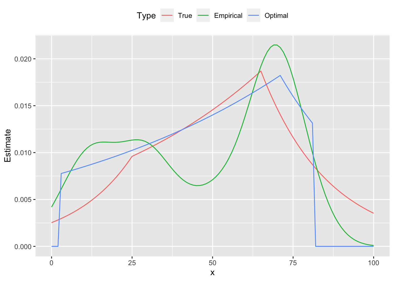
d <- data.frame(x = xrange, True = cumsum(xprobs),
                Empirical = cumsum(counts) / sum(counts),
                Optimal = cumsum(pmf))
plot.data <- gather(data = d, key = "Type", value = "Estimate", True, Empirical, Optimal,
                    factor_key = TRUE)
ggplot(plot.data) +
    geom_line(mapping = aes(x = x, y = Estimate, color = Type)) +
    theme(legend.position = "top")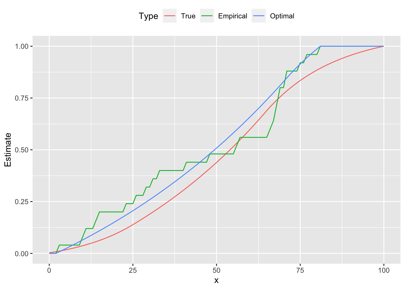
From the figures we see that the estimated curve is much closer to the true distribution, exhibiting a similar shape and number of peaks. In contrast, the empirical probability mass function oscillates, failing to be log-concave on parts of its domain. These differences are reflected in the cumulative distribution functions as well.
## Testthat Results: No output is goodSession Info
sessionInfo()## R version 4.4.2 (2024-10-31)
## Platform: x86_64-apple-darwin20
## Running under: macOS Sequoia 15.1
##
## Matrix products: default
## BLAS: /Library/Frameworks/R.framework/Versions/4.4-x86_64/Resources/lib/libRblas.0.dylib
## LAPACK: /Library/Frameworks/R.framework/Versions/4.4-x86_64/Resources/lib/libRlapack.dylib; LAPACK version 3.12.0
##
## locale:
## [1] en_US.UTF-8/en_US.UTF-8/en_US.UTF-8/C/en_US.UTF-8/en_US.UTF-8
##
## time zone: America/Los_Angeles
## tzcode source: internal
##
## attached base packages:
## [1] stats graphics grDevices datasets utils methods base
##
## other attached packages:
## [1] tidyr_1.3.1 ggplot2_3.5.1 CVXR_1.0-15 testthat_3.2.1.1
## [5] here_1.0.1
##
## loaded via a namespace (and not attached):
## [1] gmp_0.7-5 clarabel_0.9.0.1 sass_0.4.9 utf8_1.2.4
## [5] generics_0.1.3 slam_0.1-54 blogdown_1.19 lattice_0.22-6
## [9] digest_0.6.37 magrittr_2.0.3 evaluate_1.0.1 grid_4.4.2
## [13] bookdown_0.41 pkgload_1.4.0 fastmap_1.2.0 rprojroot_2.0.4
## [17] jsonlite_1.8.9 Matrix_1.7-1 ECOSolveR_0.5.5 brio_1.1.5
## [21] Rmosek_10.2.0 purrr_1.0.2 fansi_1.0.6 scales_1.3.0
## [25] codetools_0.2-20 jquerylib_0.1.4 cli_3.6.3 Rmpfr_0.9-5
## [29] rlang_1.1.4 Rglpk_0.6-5.1 bit64_4.5.2 munsell_0.5.1
## [33] withr_3.0.2 cachem_1.1.0 yaml_2.3.10 tools_4.4.2
## [37] Rcplex_0.3-6 rcbc_0.1.0.9001 dplyr_1.1.4 colorspace_2.1-1
## [41] gurobi_11.0-0 assertthat_0.2.1 vctrs_0.6.5 R6_2.5.1
## [45] lifecycle_1.0.4 bit_4.5.0 desc_1.4.3 cccp_0.3-1
## [49] pkgconfig_2.0.3 bslib_0.8.0 pillar_1.9.0 gtable_0.3.6
## [53] glue_1.8.0 Rcpp_1.0.13-1 highr_0.11 xfun_0.49
## [57] tibble_3.2.1 tidyselect_1.2.1 knitr_1.48 farver_2.1.2
## [61] htmltools_0.5.8.1 rmarkdown_2.29 labeling_0.4.3 compiler_4.4.2