L1 Trend Filtering
Introduction
Kim et al. (2009) propose the \(l_1\) trend filtering method for trend estimation. The method solves an optimization problem of the form
\[ \begin{array}{ll} \underset{\beta}{\mbox{minimize}} & \frac{1}{2}\sum_{i=1}^m (y_i - \beta_i)^2 + \lambda ||D\beta||_1 \end{array} \] where the variable to be estimated is \(\beta\) and we are given the problem data \(y\) and \(\lambda\). The matrix \(D\) is the second-order difference matrix,
\[ D = \left[ \begin{matrix} 1 & -2 & 1 & & & & \\ & 1 & -2 & 1 & & & \\ & & \ddots & \ddots & \ddots & & \\ & & & 1 & -2 & 1 & \\ & & & & 1 & -2 & 1\\ \end{matrix} \right]. \]
The implementation is in both C and Matlab. Hadley Wickham provides an R interface to the C code. This is on GitHub and can be installed via:
library(devtools)
install_github("hadley/l1tf")
Example
We will use the example in l1tf to illustrate. The package provides
the function l1tf which computes the trend estimate for a specified
\(\lambda\).
sp_data <- data.frame(x = sp500$date,
                      y = sp500$log,
                      l1_50 = l1tf(sp500$log, lambda = 50),
                      l1_100 = l1tf(sp500$log, lambda = 100))
The CVXR version
CVXR provides all the atoms and functions necessary to formulat the
problem in a few lines. For example, the \(D\) matrix above is provided
by the function diff(..., differences = 2). Notice how the
formulation tracks the mathematical construct above.
## lambda = 50
y <- sp500$log
lambda_1 <- 50
beta <- Variable(length(y))
objective_1 <- Minimize(0.5 * p_norm(y - beta) +
                        lambda_1 * p_norm(diff(x = beta, differences = 2), 1))
p1 <- Problem(objective_1)
betaHat_50 <- solve(p1)$getValue(beta)

## lambda = 100
lambda_2 <- 100
objective_2 <- Minimize(0.5 * p_norm(y - beta) +
                        lambda_2 * p_norm(diff(x = beta, differences = 2), 1))
p2 <- Problem(objective_2)
betaHat_100 <- solve(p2)$getValue(beta)
NOTE Of course, CVXR is much slower since it is not optimized just
for one problem.
## Testthat Results: No output is goodComparison Plots
A plot of the estimates for two values of \(\lambda\) is shown below
using both approaches. First the l1tf plot.
ggplot(data = sp_data) +
    geom_line(mapping = aes(x = x, y = y), color = 'grey50') +
    labs(x = "Date", y = "SP500 log-price") +
    geom_line(mapping = aes(x = x, y = l1_50), color = 'red', size = 1) +
    geom_line(mapping = aes(x = x, y = l1_100), color = 'blue', size = 1)
## Warning: Using `size` aesthetic for lines was deprecated in ggplot2 3.4.0.
## ℹ Please use `linewidth` instead.
## This warning is displayed once every 8 hours.
## Call `lifecycle::last_lifecycle_warnings()` to see where this warning was generated.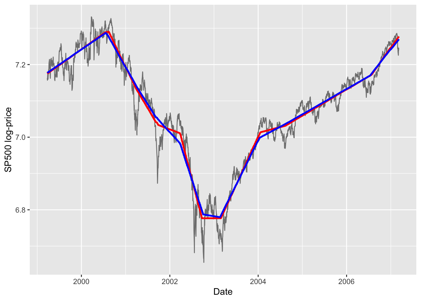
Figure 1: \(L_1\) trends for \(\lambda = 50\) (red) and \(\lambda = 100\) (blue).
Next the corresponding CVXR plots.
cvxr_data <- data.frame(x = sp500$date,
                        y = sp500$log,
                        l1_50 = betaHat_50,
                        l1_100 = betaHat_100)
ggplot(data = cvxr_data) +
    geom_line(mapping = aes(x = x, y = y), color = 'grey50') +
    labs(x = "Date", y = "SP500 log-price") +
    geom_line(mapping = aes(x = x, y = l1_50), color = 'red', size = 1) +
    geom_line(mapping = aes(x = x, y = l1_100), color = 'blue', size = 1)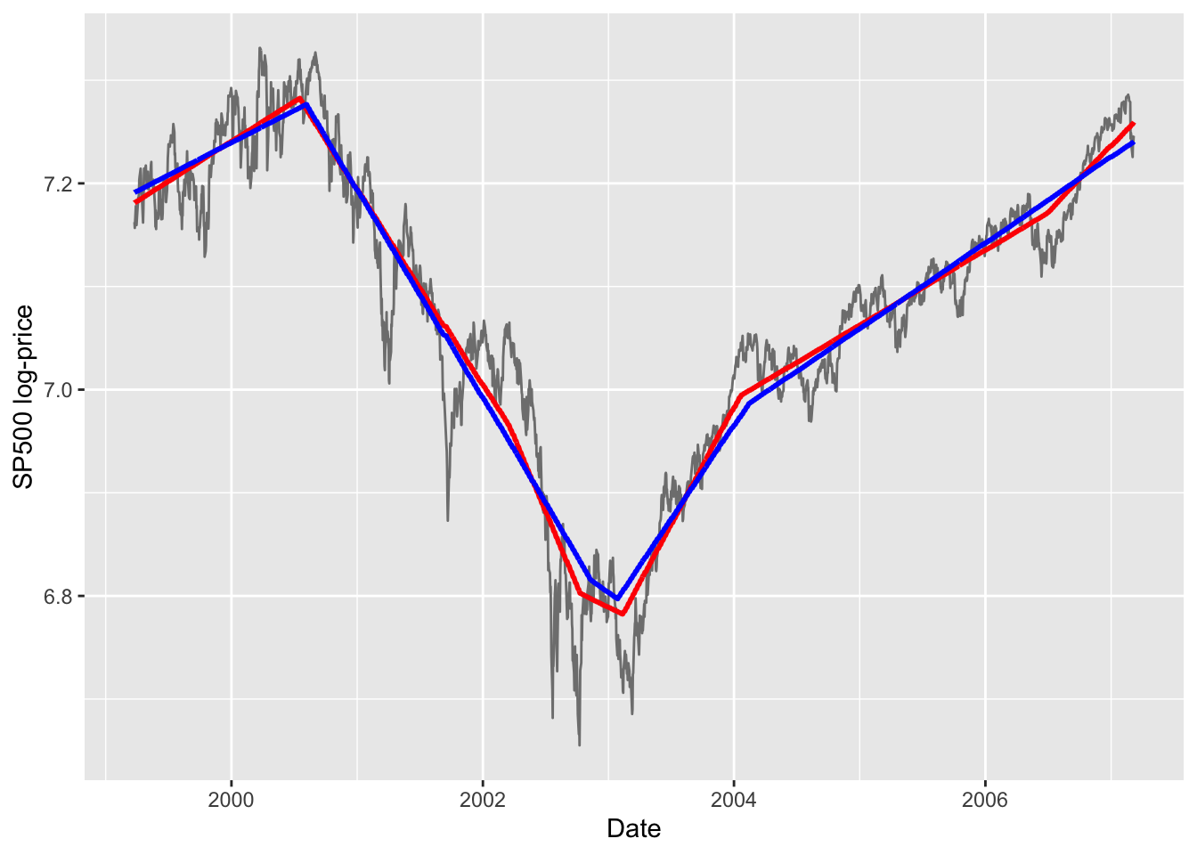
Figure 2: CVXR estimated \(L_1\) trends for \(\lambda = 50\) (red) and \(\lambda = 100\) (blue).
Notes
The CVXR solution is not quite exactly that of l1tf: on the left it shows a larger difference for the two
\(\lambda\) values; in the middle, it is less flatter than l1tf; and
on the right, it does not have as many knots as l1tf.
Session Info
sessionInfo()## R version 4.4.1 (2024-06-14)
## Platform: x86_64-apple-darwin20
## Running under: macOS Sonoma 14.5
##
## Matrix products: default
## BLAS: /Library/Frameworks/R.framework/Versions/4.4-x86_64/Resources/lib/libRblas.0.dylib
## LAPACK: /Library/Frameworks/R.framework/Versions/4.4-x86_64/Resources/lib/libRlapack.dylib; LAPACK version 3.12.0
##
## locale:
## [1] en_US.UTF-8/en_US.UTF-8/en_US.UTF-8/C/en_US.UTF-8/en_US.UTF-8
##
## time zone: America/Los_Angeles
## tzcode source: internal
##
## attached base packages:
## [1] stats graphics grDevices datasets utils methods base
##
## other attached packages:
## [1] l1tf_0.0.0.9000 ggplot2_3.5.1 CVXR_1.0-15 testthat_3.2.1.1
## [5] here_1.0.1
##
## loaded via a namespace (and not attached):
## [1] gmp_0.7-4 clarabel_0.9.0 sass_0.4.9 utf8_1.2.4
## [5] generics_0.1.3 slam_0.1-50 blogdown_1.19 lattice_0.22-6
## [9] digest_0.6.36 magrittr_2.0.3 evaluate_0.24.0 grid_4.4.1
## [13] bookdown_0.40 pkgload_1.4.0 fastmap_1.2.0 rprojroot_2.0.4
## [17] jsonlite_1.8.8 Matrix_1.7-0 ECOSolveR_0.5.5 brio_1.1.5
## [21] Rmosek_10.2.0 fansi_1.0.6 scales_1.3.0 codetools_0.2-20
## [25] jquerylib_0.1.4 cli_3.6.3 Rmpfr_0.9-5 crayon_1.5.3
## [29] rlang_1.1.4 Rglpk_0.6-5.1 bit64_4.0.5 munsell_0.5.1
## [33] withr_3.0.0 cachem_1.1.0 yaml_2.3.9 tools_4.4.1
## [37] Rcplex_0.3-6 rcbc_0.1.0.9001 dplyr_1.1.4 colorspace_2.1-0
## [41] gurobi_11.0-0 assertthat_0.2.1 vctrs_0.6.5 R6_2.5.1
## [45] lifecycle_1.0.4 bit_4.0.5 desc_1.4.3 cccp_0.3-1
## [49] pkgconfig_2.0.3 bslib_0.7.0 pillar_1.9.0 gtable_0.3.5
## [53] glue_1.7.0 Rcpp_1.0.12 highr_0.11 xfun_0.45
## [57] tibble_3.2.1 tidyselect_1.2.1 knitr_1.48 farver_2.1.2
## [61] htmltools_0.5.8.1 labeling_0.4.3 rmarkdown_2.27 compiler_4.4.1