Minimize Beamwidth of an Antenna Array

Introduction

Adapted from the CVX example of the same name, by Almir Mutapcic, 2/2/2006 and Judson Wilson, 5/14/2014.

References:

• “Convex optimization examples” lecture notes (EE364) by S. Boyd
• “Antenna array pattern synthesis via convex optimization” by H. Lebret and S. Boyd

This algorithm designs an antenna array such that:

• it has unit sensitivity at some target direction
• it obeys a constraint on a minimum sidelobe level outside the beam
• it minimizes the beamwidth of the pattern.

This is a quasiconvex problem. Define the target direction as ${\theta }_{\mathrm{tar}}$, and a beamwidth of $\mathrm{\Delta }{\theta }_{\mathrm{bw}}$. The beam occupies the angular interval

$${\mathrm{\Theta }}_b=({\theta }_{\mathrm{tar}}-\frac{1}{2}\mathrm{\Delta }{\theta }_{\mathrm{bw}},{\theta }_{\mathrm{tar}}+\frac{1}{2}\mathrm{\Delta }{\theta }_{\mathrm{bw}}).$$

Solving for the minimum beamwidth $\mathrm{\Delta }{\theta }_{\mathrm{bw}}$ is performed by bisection, where the interval which contains the optimal value is bisected according to the result of the following feasibility problem:

$$\begin{array}{ll}\text{minimize}& 0\\ \text{subject to}& y({\theta }_{\mathrm{tar}})=1\\ & |y(\theta )|\le t_{\mathrm{sb}}\mathrm{\forall }\theta \notin {\mathrm{\Theta }}_b.\end{array}$$

Here $y$ is the antenna array gain pattern (a complex-valued function), $t_{\mathrm{sb}}$ is the maximum allowed sideband gain threshold, and the variables are $w$ (antenna array weights or shading coefficients). The gain pattern is a linear function of $w$: $y(\theta )=w^{T}a(\theta )$ for some $a(\theta )$ describing the antenna array configuration and specs.

Once the optimal beamwidth is found, the solution $w$ is refined with:

$$\begin{array}{ll}\text{minimize}& \parallel w\parallel \\ \text{subject to}& y({\theta }_{\mathrm{tar}})=1\\ & |y(\theta )|\le t_{\mathrm{sb}}\mathrm{\forall }\theta \notin {\mathrm{\Theta }}_b.\end{array}$$

The implementation below discretizes the angular quantities.

Problem Data

We use a random 2D positioning of antennas.

## Problem specs
lambda_wl <- 1         # wavelength
theta_tar <- 60        # target direction (degrees)
min_sidelobe <- -20    # maximum sidelobe level in dB
max_half_beam <- 50    # starting half beamwidth (must be feasible)

## 2D random antenna locations
set.seed(1)
n <- 36
L <- 5
loc <- matrix(L * runif(n * 2), nrow = n, ncol = 2)

Build Optimization Matrices

We construct the matrix $A$ that relates the weights $w$ and the gain pattern $y(\theta )$, i.e., $y=Aw$.

## Theta in degrees from 1 to 360
theta <- matrix(1:360, ncol = 1)

## Build matrix A: y = A * w (complex-valued)
A <- exp(2i * pi / lambda_wl *
         (cos(pi * theta / 180) %*% t(loc[, 1]) +
          sin(pi * theta / 180) %*% t(loc[, 2])))

## Target constraint
ind_closest <- which.min(abs(theta - theta_tar))
Atar <- A[ind_closest, , drop = FALSE]

Solve Using Bisection

Since CVXR works with real variables, we represent complex-valued quantities by separating real and imaginary parts. A complex vector $w=w_R+i{w}_I$ is stored as a real vector $(w_R,w_I)$.

## Set up real/imaginary representation of Atar
Atar_R <- Re(Atar)
Atar_I <- Im(Atar)
Atar_RI <- rbind(cbind(Atar_R, -Atar_I),
                 cbind(Atar_I,  Atar_R))

## Target vector: [1, 0] (unit gain, no imaginary component)
realones_ri <- c(1.0, 0.0)

## Bisection
halfbeam_bot <- 1
halfbeam_top <- max_half_beam

cat("We are only considering integer values of the half beam-width\n")
cat("(since we are sampling the angle with 1 degree resolution).\n\n")

while (halfbeam_top - halfbeam_bot > 1) {
    halfbeam_cur <- ceiling((halfbeam_top + halfbeam_bot) / 2)

    ## Indices of the stopband (outside the beam)
    ind <- which(theta <= (theta_tar - halfbeam_cur) |
                 theta >= (theta_tar + halfbeam_cur))
    As <- A[ind, , drop = FALSE]

    ## Real/imaginary representation
    As_R <- Re(As)
    As_I <- Im(As)
    As_RI_top <- cbind(As_R, -As_I)
    As_RI_bot <- cbind(As_I,  As_R)

    ## CVXR variables and constraints
    w_ri <- Variable(2 * n)
    constraints <- list(Atar_RI %*% w_ri == realones_ri)

    ## Add sidelobe constraints row by row
    sidelobe_thresh <- 10^(min_sidelobe / 20)
    sidelobe_constraints <- lapply(seq_len(nrow(As)), function(i) {
        As_ri_row <- rbind(As_RI_top[i, , drop = FALSE],
                           As_RI_bot[i, , drop = FALSE])
        p_norm(As_ri_row %*% w_ri, 2) <= sidelobe_thresh
    })
    constraints <- c(constraints, sidelobe_constraints)

    ## Solve feasibility problem
    obj <- Minimize(0)
    prob <- Problem(obj, constraints)
    result <- psolve(prob, solver = "SCS")

    ## Bisection logic
    if (status(prob) == "optimal") {
        cat(sprintf("Problem is feasible for half beam-width = %g degrees\n",
                    halfbeam_cur))
        halfbeam_top <- halfbeam_cur
    } else {
        cat(sprintf("Problem is not feasible for half beam-width = %g degrees\n",
                    halfbeam_cur))
        halfbeam_bot <- halfbeam_cur
    }
}

halfbeam <- halfbeam_top
cat(sprintf("\nOptimum half beam-width for given specs is %g degrees\n", halfbeam))

We are only considering integer values of the half beam-width
(since we are sampling the angle with 1 degree resolution).

Problem is feasible for half beam-width = 26 degrees
Problem is feasible for half beam-width = 14 degrees
Problem is not feasible for half beam-width = 8 degrees
Problem is feasible for half beam-width = 11 degrees
Problem is feasible for half beam-width = 10 degrees
Problem is not feasible for half beam-width = 9 degrees

Optimum half beam-width for given specs is 10 degrees

Minimum Noise Design

We now compute the minimum-norm weights for the optimal beamwidth.

## Recompute stopband for optimal beamwidth
ind <- which(theta <= (theta_tar - halfbeam) |
             theta >= (theta_tar + halfbeam))
As <- A[ind, , drop = FALSE]

As_R <- Re(As)
As_I <- Im(As)
As_RI_top <- cbind(As_R, -As_I)
As_RI_bot <- cbind(As_I,  As_R)

w_ri <- Variable(2 * n)
constraints <- list(Atar_RI %*% w_ri == realones_ri)

sidelobe_thresh <- 10^(min_sidelobe / 20)
sidelobe_constraints <- lapply(seq_len(nrow(As)), function(i) {
    As_ri_row <- rbind(As_RI_top[i, , drop = FALSE],
                       As_RI_bot[i, , drop = FALSE])
    p_norm(As_ri_row %*% w_ri, 2) <= sidelobe_thresh
})
constraints <- c(constraints, sidelobe_constraints)

## Minimize the weight norm
obj <- Minimize(p_norm(w_ri, 2))
prob <- Problem(obj, constraints)
result_final <- psolve(prob, solver = "SCS")
cat(sprintf("Final objective value: %f\n", result_final))

Final objective value: 0.277997

Result Plots

Antenna Locations

ggplot(data.frame(x = loc[, 1], y = loc[, 2])) +
    geom_point(aes(x = x, y = y), shape = 1, size = 3, color = "blue") +
    labs(title = "Antenna Locations", x = "x", y = "y") +
    coord_fixed() +
    theme_minimal()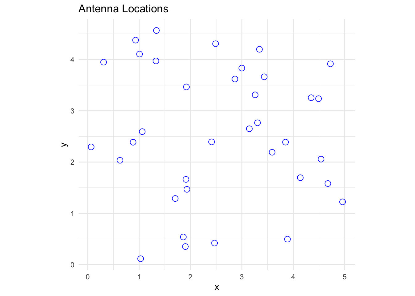

Antenna locations in 2D plane

Array Pattern

## Compute full gain pattern
A_R <- Re(A)
A_I <- Im(A)
A_RI <- rbind(cbind(A_R, -A_I), cbind(A_I, A_R))

w_ri_val <- value(w_ri)
y_full <- A_RI %*% w_ri_val
n_theta <- length(theta)
y_complex <- y_full[1:n_theta] + 1i * y_full[(n_theta + 1):(2 * n_theta)]
y_mag_db <- 20 * log10(abs(y_complex))

df_pattern <- data.frame(
    theta = as.vector(theta),
    gain_db = as.vector(y_mag_db)
)

ggplot(df_pattern, aes(x = theta, y = gain_db)) +
    geom_line() +
    geom_vline(xintercept = theta_tar, linetype = "dashed", color = "green") +
    geom_vline(xintercept = theta_tar + halfbeam, linetype = "dashed", color = "red") +
    geom_vline(xintercept = theta_tar - halfbeam, linetype = "dashed", color = "red") +
    ylim(-40, 0) +
    labs(x = "Look angle (degrees)", y = "Magnitude (dB)",
         title = "Array Gain Pattern") +
    theme_minimal()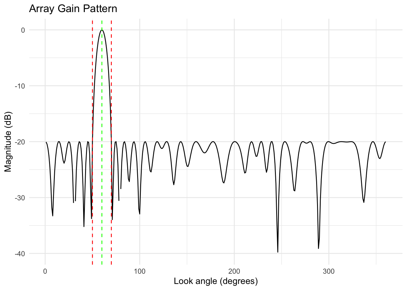

Array gain pattern in dB

Polar Pattern

zerodB <- 50
dBY <- pmax(y_mag_db + zerodB, 0)
theta_rad <- as.vector(theta) * pi / 180

df_polar <- data.frame(
    x = as.vector(dBY) * cos(theta_rad),
    y = as.vector(dBY) * sin(theta_rad)
)

## 0 dB circle
circle_0dB <- data.frame(
    x = zerodB * cos(theta_rad),
    y = zerodB * sin(theta_rad)
)

## Sidelobe circle
m_sl <- min_sidelobe + zerodB
circle_sl <- data.frame(
    x = m_sl * cos(theta_rad),
    y = m_sl * sin(theta_rad)
)

ggplot() +
    geom_path(data = df_polar, aes(x = x, y = y), color = "blue") +
    geom_path(data = circle_0dB, aes(x = x, y = y), linetype = "dotted") +
    geom_path(data = circle_sl, aes(x = x, y = y), linetype = "dotted") +
    coord_fixed(xlim = c(-zerodB, zerodB), ylim = c(-zerodB, zerodB)) +
    annotate("text", x = -zerodB, y = 2, label = "0 dB") +
    annotate("text", x = -m_sl, y = 2, label = paste0(min_sidelobe, " dB")) +
    labs(title = "Polar Radiation Pattern") +
    theme_void()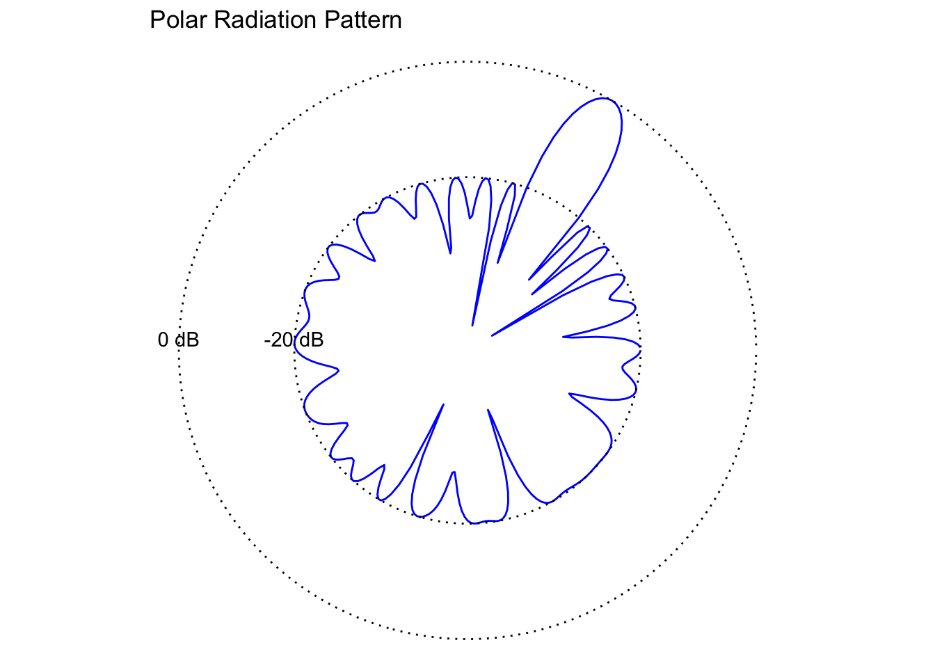

Polar radiation pattern

Session Info

R version 4.5.2 (2025-10-31)
Platform: aarch64-apple-darwin20
Running under: macOS Tahoe 26.3

Matrix products: default
BLAS:   /Library/Frameworks/R.framework/Versions/4.5-arm64/Resources/lib/libRblas.0.dylib 
LAPACK: /Library/Frameworks/R.framework/Versions/4.5-arm64/Resources/lib/libRlapack.dylib;  LAPACK version 3.12.1

locale:
[1] en_US.UTF-8/en_US.UTF-8/en_US.UTF-8/C/en_US.UTF-8/en_US.UTF-8

time zone: America/Los_Angeles
tzcode source: internal

attached base packages:
[1] stats     graphics  grDevices utils     datasets  methods   base     

other attached packages:
[1] ggplot2_4.0.2 CVXR_1.8.1   

loaded via a namespace (and not attached):
 [1] gmp_0.7-5.1        generics_0.1.4     clarabel_0.11.2    slam_0.1-55       
 [5] lattice_0.22-9     digest_0.6.39      magrittr_2.0.4     evaluate_1.0.5    
 [9] grid_4.5.2         RColorBrewer_1.1-3 fastmap_1.2.0      jsonlite_2.0.0    
[13] Matrix_1.7-4       ECOSolveR_0.6.1    backports_1.5.0    scs_3.2.7         
[17] Rmosek_11.1.1      scales_1.4.0       codetools_0.2-20   cli_3.6.5         
[21] rlang_1.1.7        Rglpk_0.6-5.1      withr_3.0.2        yaml_2.3.12       
[25] otel_0.2.0         tools_4.5.2        osqp_1.0.0         Rcplex_0.3-8      
[29] checkmate_2.3.4    dplyr_1.2.0        gurobi_13.0-1      vctrs_0.7.1       
[33] R6_2.6.1           lifecycle_1.0.5    htmlwidgets_1.6.4  pkgconfig_2.0.3   
[37] cccp_0.3-3         pillar_1.11.1      gtable_0.3.6       glue_1.8.0        
[41] Rcpp_1.1.1         xfun_0.56          tibble_3.3.1       tidyselect_1.2.1  
[45] knitr_1.51         dichromat_2.0-0.1  highs_1.12.0-3     farver_2.1.2      
[49] htmltools_0.5.9    rmarkdown_2.30     labeling_0.4.3     piqp_0.6.2        
[53] compiler_4.5.2     S7_0.2.1          

References