elastic_reg <- function(beta, lambda = 0, alpha = 0) {
    ridge <- (1 - alpha) / 2 * sum_squares(beta)
    lasso <- alpha * p_norm(beta, 1)
    lambda * (lasso + ridge)
}Elastic Net
Introduction
Often in applications, we encounter problems that require regularization to prevent overfitting, introduce sparsity, facilitate variable selection, or impose prior distributions on parameters. Two of the most common regularization functions are the \(l_1\)-norm and squared \(l_2\)-norm, combined in the elastic net regression model Friedman et al. (2010),
\[ \begin{array}{ll} \underset{\beta}{\mbox{minimize}} & \frac{1}{2m}\|y - X\beta\|_2^2 + \lambda(\frac{1-\alpha}{2}\|\beta\|_2^2 + \alpha\|\beta\|_1). \end{array} \]
Here \(\lambda \geq 0\) is the overall regularization weight and \(\alpha \in [0,1]\) controls the relative \(l_1\) versus squared \(l_2\) penalty. Thus, this model encompasses both ridge (\(\alpha = 0\)) and lasso (\(\alpha = 1\)) regression.
Example
To solve this problem in CVXR, we first define a function that calculates the regularization term given the variable and penalty weights.
Later, we will add it to the scaled least squares loss as shown below.
loss <- sum_squares(y - X %*% beta) / (2 * n)
obj <- loss + elastic_reg(beta, lambda, alpha)
The advantage of this modular approach is that we can easily incorporate elastic net regularization into other regression models. For instance, if we wanted to run regularized Huber regression, CVXR allows us to reuse the above code with just a single changed line.
loss <- huber(y - X %*% beta, M)We generate some synthetic sparse data for this example. We use correlated features (Toeplitz structure with \(\rho = 0.8\)) and set \(n = 100\), \(p = 50\) so that regularization is essential. Correlated features are the classic motivation for elastic net over pure lasso: lasso tends to pick one variable from a correlated group arbitrarily, while elastic net encourages the group to enter or leave together.
We also scale \(y\) so that \(\sqrt{\text{mean}(y^2)} = 1\). The reason is explained in the glmnet comparison below.
set.seed(1)

# Problem data
p <- 50
n <- 100

# Correlated features: Toeplitz covariance Sigma_ij = rho^|i-j|
rho <- 0.8
Sigma <- rho^abs(outer(seq_len(p), seq_len(p), "-"))
X <- MASS::mvrnorm(n, mu = rep(0, p), Sigma = Sigma)

# Sparse true coefficients: 10 non-zero with varying magnitudes
beta_true <- rep(0, p)
beta_true[c(1, 5, 10, 15, 20, 25, 30, 35, 40, 45)] <-
    c(3, -2.5, 2, -1.5, 1, -3, 2.5, -2, 1.5, -1)

# Noise calibrated for SNR ~ 3
signal_sd <- sqrt(drop(t(beta_true) %*% Sigma %*% beta_true))
sigma <- signal_sd / 3
y <- X %*% beta_true + rnorm(n, sd = sigma)

# Scale y so that sqrt(mean(y^2)) = 1
y <- y / sqrt(mean(y^2))
We fit the elastic net model for several values of \(\lambda\).
TRIALS <- 10
lambda_vals <- 10^seq(-2, 0, length.out = TRIALS)
beta <- Variable(p)
loss <- sum_squares(y - X %*% beta) / (2 * n)

## Elastic-net regression
alpha <- 0.75
beta_vals <- sapply(lambda_vals,
                    function(lambda) {
                        obj <- loss + elastic_reg(beta, lambda, alpha)
                        prob <- Problem(Minimize(obj))
                        psolve(prob)
                        check_solver_status(prob)
                        value(beta)
                    })
We can now get a table of the coefficients. With \(p = 50\) coefficients, we show only the 10 that correspond to the true non-zero entries.
nz_idx <- which(beta_true != 0)
d <- as.data.frame(beta_vals[nz_idx, ])
rownames(d) <- sprintf("\\(\\beta_{%d}\\)", nz_idx)
names(d) <- sprintf("\\(\\lambda = %.3f\\)", lambda_vals)
knitr::kable(d, format = "html", escape = FALSE, caption = "Elastic net fits from <code>CVXR</code> (non-zero coefficients)", digits = 3) |>
    kable_styling("striped") |>
column_spec(1:11, background = "#ececec")| \(\lambda = 0.010\) | \(\lambda = 0.017\) | \(\lambda = 0.028\) | \(\lambda = 0.046\) | \(\lambda = 0.077\) | \(\lambda = 0.129\) | \(\lambda = 0.215\) | \(\lambda = 0.359\) | \(\lambda = 0.599\) | \(\lambda = 1.000\) | |
|---|---|---|---|---|---|---|---|---|---|---|
| \(\beta_{1}\) | 0.517 | 0.510 | 0.499 | 0.479 | 0.438 | 0.361 | 0.256 | 0.115 | 0 | 0 |
| \(\beta_{5}\) | -0.504 | -0.487 | -0.481 | -0.475 | -0.441 | -0.389 | -0.277 | -0.142 | 0 | 0 |
| \(\beta_{10}\) | 0.258 | 0.250 | 0.252 | 0.249 | 0.206 | 0.118 | 0.000 | 0.000 | 0 | 0 |
| \(\beta_{15}\) | -0.192 | -0.184 | -0.166 | -0.147 | -0.095 | -0.025 | 0.000 | 0.000 | 0 | 0 |
| \(\beta_{20}\) | 0.192 | 0.165 | 0.135 | 0.097 | 0.046 | 0.000 | 0.000 | 0.000 | 0 | 0 |
| \(\beta_{25}\) | -0.695 | -0.640 | -0.577 | -0.525 | -0.450 | -0.362 | -0.255 | -0.102 | 0 | 0 |
| \(\beta_{30}\) | 0.595 | 0.548 | 0.500 | 0.443 | 0.379 | 0.282 | 0.129 | 0.000 | 0 | 0 |
| \(\beta_{35}\) | -0.290 | -0.290 | -0.279 | -0.262 | -0.215 | -0.142 | -0.055 | 0.000 | 0 | 0 |
| \(\beta_{40}\) | 0.130 | 0.136 | 0.135 | 0.123 | 0.072 | 0.000 | 0.000 | 0.000 | 0 | 0 |
| \(\beta_{45}\) | -0.158 | -0.138 | -0.117 | -0.085 | -0.043 | 0.000 | 0.000 | 0.000 | 0 | 0 |
We plot the regularization path for all coefficients. With correlated features and \(n\) only twice \(p\), the coefficients sweep dramatically from their unregularized values down to zero as \(\lambda\) increases.
df_path <- data.frame(lambda = lambda_vals, t(beta_vals)) |>
    pivot_longer(-lambda, names_to = "Coefficient", values_to = "Value")
ggplot(df_path, aes(x = lambda, y = Value, color = Coefficient)) +
    geom_line() +
    scale_x_log10() +
    labs(x = expression(lambda), y = expression(beta),
         title = "Regularization Path for Elastic-net Regression") +
    theme_minimal() +
    guides(color = "none")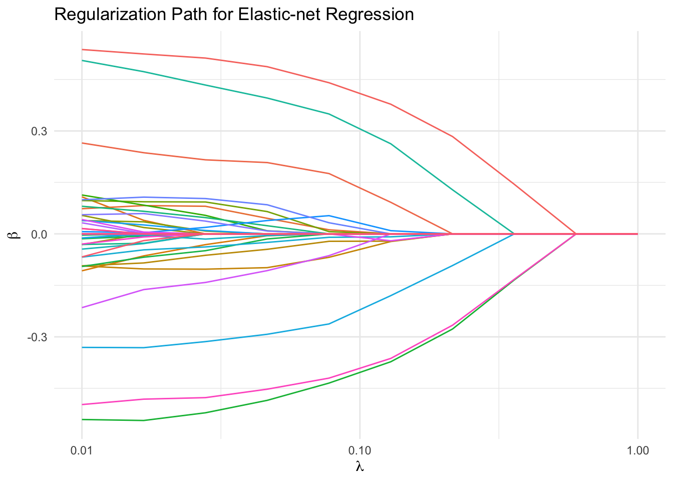
Comparison with glmnet
We can compare with results from glmnet. One subtlety: for the Gaussian family with intercept = FALSE, glmnet internally divides \(y\) by \(s = \sqrt{\text{mean}(y^2)}\) before fitting, then rescales the returned coefficients by \(s\). Because the internal fit uses \(\tilde{y}
= y/s\) while the penalty is unchanged, the \(l_1\) and \(l_2\) terms in the elastic net get reweighted by different powers of \(s\). No single \(\lambda\)-correction can undo this when \(\alpha \in (0, 1)\).
The simplest fix is to ensure \(s = 1\) so the standardization is a no-op, which is why we scaled \(y\) above. With that in place, the same \(\lambda\) values give both methods the same effective problem.
model_net <- glmnet(X, y, family = "gaussian", alpha = alpha,
                    lambda = lambda_vals, standardize = FALSE,
                    intercept = FALSE)
## glmnet returns columns in decreasing lambda order; reverse to match
coef_net <- as.data.frame(as.matrix(coef(model_net)[-1, seq(TRIALS, 1, by = -1)]))
d_net <- coef_net[nz_idx, ]
rownames(d_net) <- sprintf("\\(\\beta_{%d}\\)", nz_idx)
names(d_net) <- sprintf("\\(\\lambda = %.3f\\)", lambda_vals)
knitr::kable(d_net, format = "html", escape = FALSE, digits = 3, caption = "Coefficients from <code>glmnet</code> (non-zero coefficients)") |>
    kable_styling("striped") |>
column_spec(1:11, background = "#ececec")| \(\lambda = 0.010\) | \(\lambda = 0.017\) | \(\lambda = 0.028\) | \(\lambda = 0.046\) | \(\lambda = 0.077\) | \(\lambda = 0.129\) | \(\lambda = 0.215\) | \(\lambda = 0.359\) | \(\lambda = 0.599\) | \(\lambda = 1.000\) | |
|---|---|---|---|---|---|---|---|---|---|---|
| \(\beta_{1}\) | 0.517 | 0.510 | 0.499 | 0.480 | 0.438 | 0.361 | 0.256 | 0.115 | 0 | 0 |
| \(\beta_{5}\) | -0.503 | -0.487 | -0.481 | -0.475 | -0.441 | -0.389 | -0.277 | -0.142 | 0 | 0 |
| \(\beta_{10}\) | 0.258 | 0.250 | 0.252 | 0.249 | 0.206 | 0.118 | 0.000 | 0.000 | 0 | 0 |
| \(\beta_{15}\) | -0.192 | -0.184 | -0.167 | -0.147 | -0.095 | -0.025 | 0.000 | 0.000 | 0 | 0 |
| \(\beta_{20}\) | 0.192 | 0.165 | 0.135 | 0.097 | 0.046 | 0.000 | 0.000 | 0.000 | 0 | 0 |
| \(\beta_{25}\) | -0.695 | -0.639 | -0.577 | -0.525 | -0.450 | -0.362 | -0.255 | -0.102 | 0 | 0 |
| \(\beta_{30}\) | 0.595 | 0.548 | 0.500 | 0.443 | 0.379 | 0.282 | 0.129 | 0.000 | 0 | 0 |
| \(\beta_{35}\) | -0.290 | -0.290 | -0.279 | -0.262 | -0.214 | -0.142 | -0.055 | 0.000 | 0 | 0 |
| \(\beta_{40}\) | 0.130 | 0.136 | 0.135 | 0.123 | 0.072 | 0.000 | 0.000 | 0.000 | 0 | 0 |
| \(\beta_{45}\) | -0.158 | -0.138 | -0.117 | -0.085 | -0.043 | 0.000 | 0.000 | 0.000 | 0 | 0 |
Session Info
R version 4.6.0 (2026-04-24)
Platform: aarch64-apple-darwin23
Running under: macOS Tahoe 26.5.1

Matrix products: default
BLAS:   /Library/Frameworks/R.framework/Versions/4.6/Resources/lib/libRblas.0.dylib
LAPACK: /Library/Frameworks/R.framework/Versions/4.6/Resources/lib/libRlapack.dylib;  LAPACK version 3.12.1

locale:
[1] en_US.UTF-8/en_US.UTF-8/en_US.UTF-8/C/en_US.UTF-8/en_US.UTF-8

time zone: America/Los_Angeles
tzcode source: internal

attached base packages:
[1] stats     graphics  grDevices utils     datasets  methods   base

other attached packages:
[1] glmnet_5.0       Matrix_1.7-5     kableExtra_1.4.0 tidyr_1.3.2
[5] ggplot2_4.0.3    CVXR_1.9.1

loaded via a namespace (and not attached):
 [1] gtable_0.3.6       shape_1.4.6.1      xfun_0.58          htmlwidgets_1.6.4
 [5] lattice_0.22-9     vctrs_0.7.3        tools_4.6.0        generics_0.1.4
 [9] tibble_3.3.1       highs_1.14.0-2     pkgconfig_2.0.3    piqp_0.6.2
[13] checkmate_2.3.4    RColorBrewer_1.1-3 S7_0.2.2           lifecycle_1.0.5
[17] compiler_4.6.0     farver_2.1.2       stringr_1.6.0      textshaping_1.0.5
[21] codetools_0.2-20   ECOSolveR_0.6.1    htmltools_0.5.9    cccp_0.3-3
[25] yaml_2.3.12        gmp_0.7-5.1        pillar_1.11.1      MASS_7.3-65
[29] clarabel_0.11.2    iterators_1.0.14   foreach_1.5.2      tidyselect_1.2.1
[33] digest_0.6.39      stringi_1.8.7      slam_0.1-55        dplyr_1.2.1
[37] purrr_1.2.2        labeling_0.4.3     splines_4.6.0      rprojroot_2.1.1
[41] fastmap_1.2.0      grid_4.6.0         here_1.0.2         cli_3.6.6
[45] magrittr_2.0.5     dichromat_2.0-0.1  survival_3.8-6     withr_3.0.2
[49] scales_1.4.0       backports_1.5.1    rmarkdown_2.31     scs_3.2.7
[53] otel_0.2.0         evaluate_1.0.5     knitr_1.51         Rglpk_0.6-5.1
[57] viridisLite_0.4.3  rlang_1.2.0        Rcpp_1.1.1-1.1     glue_1.8.1
[61] xml2_1.5.2         osqp_1.0.0         svglite_2.2.2      rstudioapi_0.18.0
[65] jsonlite_2.0.0     R6_2.6.1           systemfonts_1.3.2
References
Friedman, J., T. Hastie, and R. Tibshirani. 2010. “Regularization Paths for Generalized Linear Models via Coordinate Descent.” Journal of Statistical Software 33 (1): 1–22.
H. Zou, T. Hastie. 2005. “Regularization and Variable Selection via the Elastic–Net.” Journal of the Royal Statistical Society. Series B (Methodological) 67 (2): 301–20.