set.seed(1)
n <- 20
m <- 1000
TEST <- m
DENSITY <- 0.2

beta_true <- rnorm(n)
idxs <- sample.int(n, size = as.integer((1 - DENSITY) * n), replace = FALSE)
beta_true[idxs] <- 0
offset <- 0
sigma <- 45

X <- matrix(rnorm(m * n, sd = 5), nrow = m, ncol = n)
Y <- as.vector(sign(X %*% beta_true + offset + rnorm(m, sd = sigma)))
X_test <- matrix(rnorm(TEST * n, sd = 5), nrow = TEST, ncol = n)
Y_test <- as.vector(sign(X_test %*% beta_true + offset + rnorm(TEST, sd = sigma)))Support Vector Machine with l1 Regularization
Introduction
In this example we use CVXR to train an SVM classifier with \(\ell_1\)-regularization. We are given data \((x_i, y_i)\), \(i = 1, \ldots, m\). The \(x_i \in \mathbf{R}^n\) are feature vectors, while the \(y_i \in \{\pm 1\}\) are associated boolean outcomes. Our goal is to construct a good linear classifier \(\hat{y} = \text{sign}(\beta^T x - v)\). We find the parameters \(\beta, v\) by minimizing the (convex) function
\[ f(\beta, v) = \frac{1}{m} \sum_i \left(1 - y_i (\beta^T x_i - v)\right)_+ + \lambda \|\beta\|_1. \]
The first term is the average hinge loss. The second term shrinks the coefficients in \(\beta\) and encourages sparsity. The scalar \(\lambda \geq 0\) is a (regularization) parameter. Minimizing \(f(\beta, v)\) simultaneously selects features and fits the classifier.
Example
In the following code we generate data with \(n = 20\) features by randomly choosing \(x_i\) and a sparse \(\beta_{\text{true}} \in \mathbf{R}^n\). We then set \(y_i = \text{sign}(\beta_{\text{true}}^T x_i - v_{\text{true}} - z_i)\), where the \(z_i\) are i.i.d. normal random variables. We divide the data into training and test sets with \(m = 1000\) examples each.
We next formulate the optimization problem using CVXR.
beta  <- Variable(n)
v     <- Variable()
loss  <- sum_entries(pos(1 - Y * (X %*% beta - v)))
reg   <- p_norm(beta, 1)
We solve the optimization problem for a range of \(\lambda\) to compute a trade-off curve. We then plot the train and test error over the trade-off curve. A reasonable choice of \(\lambda\) is the value that minimizes the test error.
TRIALS <- 100
train_error <- numeric(TRIALS)
test_error  <- numeric(TRIALS)
lambda_vals <- 10^seq(-2, 0, length.out = TRIALS)
beta_vals   <- vector("list", TRIALS)

for (i in seq_len(TRIALS)) {
    prob <- Problem(Minimize(loss / m + lambda_vals[i] * reg))
    result <- psolve(prob)
    check_solver_status(prob)
    beta_hat <- drop(value(beta))
    v_hat    <- drop(value(v))
    train_error[i] <- sum(sign(X %*% beta_true + offset) !=
                          sign(X %*% beta_hat - v_hat)) / m
    test_error[i]  <- sum(sign(X_test %*% beta_true + offset) !=
                          sign(X_test %*% beta_hat - v_hat)) / TEST
    beta_vals[[i]] <- beta_hat
}
df_error <- data.frame(lambda = lambda_vals,
Train = train_error,
Test = test_error) |>
pivot_longer(-lambda, names_to = "Set", values_to = "Error")
ggplot(df_error, aes(x = lambda, y = Error, color = Set)) +
geom_line() +
scale_x_log10() +
scale_color_manual(values = c(Train = "blue", Test = "red")) +
labs(x = expression(lambda), y = "Classification Error",
title = "Train vs. Test Error") +
theme_minimal()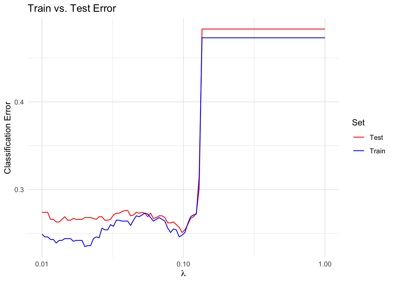
Regularization Path
We also plot the regularization path, or the \(\beta_i\) versus \(\lambda\). Notice that the \(\beta_i\) do not necessarily decrease monotonically as \(\lambda\) increases. Four features remain non-zero longer for larger \(\lambda\) than the rest, which suggests that these features are the most important. In fact \(\beta_{\text{true}}\) had 4 non-zero values.
beta_mat <- do.call(cbind, lapply(beta_vals, as.vector))
df_path <- data.frame(lambda = lambda_vals, t(beta_mat)) |>
    pivot_longer(-lambda, names_to = "Coefficient", values_to = "Value")
ggplot(df_path, aes(x = lambda, y = Value, color = Coefficient)) +
    geom_line() +
    scale_x_log10() +
    labs(x = expression(lambda), y = expression(beta[i]),
         title = "Regularization Path") +
    theme_minimal() +
    guides(color = "none")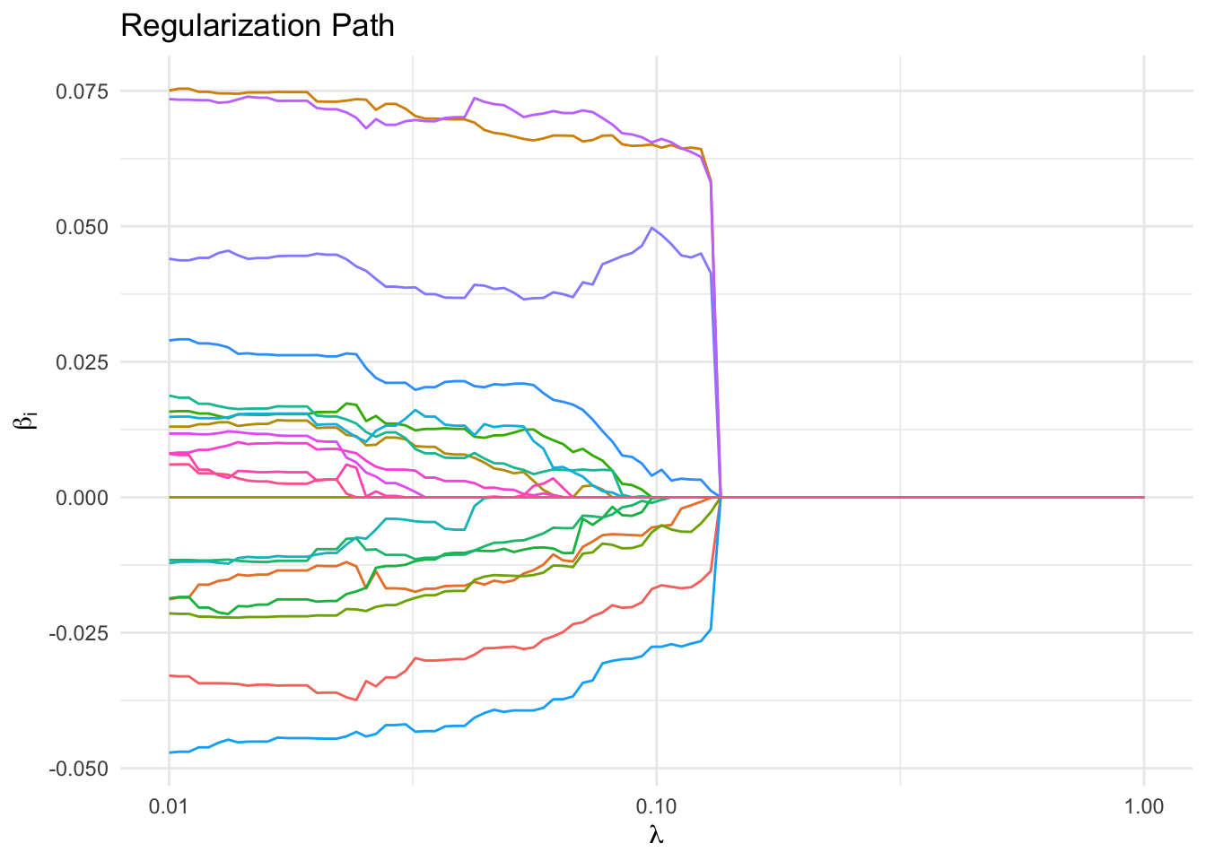
Session Info
R version 4.6.0 (2026-04-24)
Platform: aarch64-apple-darwin23
Running under: macOS Tahoe 26.5.1

Matrix products: default
BLAS:   /Library/Frameworks/R.framework/Versions/4.6/Resources/lib/libRblas.0.dylib
LAPACK: /Library/Frameworks/R.framework/Versions/4.6/Resources/lib/libRlapack.dylib;  LAPACK version 3.12.1

locale:
[1] en_US.UTF-8/en_US.UTF-8/en_US.UTF-8/C/en_US.UTF-8/en_US.UTF-8

time zone: America/Los_Angeles
tzcode source: internal

attached base packages:
[1] stats     graphics  grDevices utils     datasets  methods   base

other attached packages:
[1] tidyr_1.3.2   ggplot2_4.0.3 CVXR_1.9.1

loaded via a namespace (and not attached):
 [1] gmp_0.7-5.1        generics_0.1.4     clarabel_0.11.2    slam_0.1-55
 [5] lattice_0.22-9     digest_0.6.39      magrittr_2.0.5     evaluate_1.0.5
 [9] grid_4.6.0         RColorBrewer_1.1-3 fastmap_1.2.0      rprojroot_2.1.1
[13] jsonlite_2.0.0     Matrix_1.7-5       ECOSolveR_0.6.1    backports_1.5.1
[17] scs_3.2.7          purrr_1.2.2        scales_1.4.0       codetools_0.2-20
[21] cli_3.6.6          rlang_1.2.0        Rglpk_0.6-5.1      withr_3.0.2
[25] yaml_2.3.12        otel_0.2.0         tools_4.6.0        osqp_1.0.0
[29] checkmate_2.3.4    dplyr_1.2.1        here_1.0.2         vctrs_0.7.3
[33] R6_2.6.1           lifecycle_1.0.5    htmlwidgets_1.6.4  pkgconfig_2.0.3
[37] cccp_0.3-3         pillar_1.11.1      gtable_0.3.6       glue_1.8.1
[41] Rcpp_1.1.1-1.1     xfun_0.58          tibble_3.3.1       tidyselect_1.2.1
[45] knitr_1.51         dichromat_2.0-0.1  highs_1.14.0-2     farver_2.1.2
[49] htmltools_0.5.9    rmarkdown_2.31     labeling_0.4.3     piqp_0.6.2
[53] compiler_4.6.0     S7_0.2.2