water_filling <- function(n, a, sum_x = 1) {
    ## Boyd and Vandenberghe, Convex Optimization, example 5.2 page 145
    ## Water-filling.
    ##
    ## This problem arises in information theory, in allocating power to a
    ## set of n communication channels in order to maximize the total
    ## channel capacity. The variable x_i represents the transmitter power
    ## allocated to the ith channel, and log(alpha_i + x_i) gives the
    ## capacity or maximum communication rate of the channel. The objective
    ## is to maximize sum(log(alpha_i + x_i)) subject to sum(x_i) = sum_x.

    ## Declare variables and parameters
    x <- Variable(n)
    alpha <- a

    ## Objective: maximize the total communication rate
    obj <- Maximize(sum(log(alpha + x)))

    ## Constraints
    constraints <- list(x >= 0, sum(x) == sum_x)

    ## Solve
    prob <- Problem(obj, constraints)
    result <- psolve(prob)

    prob_status <- status(prob)
    if (prob_status == "optimal") {
        list(status = prob_status,
             value = result,
             x = as.vector(value(x)))
    } else {
        list(status = prob_status,
             value = NA,
             x = NA)
    }
}Water Filling in Communications
Introduction
From Boyd and Vandenberghe, Convex Optimization, Example 5.2 (page 145).
Convex optimization can be used to solve the classic water filling problem. This problem is where a total amount of power \(P\) has to be assigned to \(n\) communication channels, with the objective of maximizing the total communication rate. The communication rate of the \(i\)th channel is given by
\[ \log(\alpha_i + x_i) \]
where \(x_i\) represents the power allocated to channel \(i\) and \(\alpha_i\) represents the floor above the baseline at which power can be added to the channel. Since \(-\log(X)\) is convex, we can write the water-filling problem as a convex optimization problem:
\[ \begin{array}{ll} \mbox{minimize} & \sum_{i=1}^{N} -\log(\alpha_i + x_i) \\ \mbox{subject to} & x_i \geq 0, \quad \sum_{i=1}^{N} x_i = P \end{array} \]
This form is straightforward to express in DCP format and thus can be simply solved using CVXR.
Water Filling Function
We define a function that solves the water-filling problem for given channel parameters and total power budget.
Example
As a simple example, we set \(N = 3\), \(P = 1\) and \(\boldsymbol{\alpha} = (0.8, 1.0, 1.2)\).
The function outputs the problem status, the maximum communication rate, and the power allocation required to achieve this maximum communication rate.
buckets <- 3
alpha <- c(0.8, 1.0, 1.2)

sol <- water_filling(buckets, alpha)
cat("Problem status:", sol$status, "\n")
cat(sprintf("Optimal communication rate = %.4g\n", sol$value))
cat("Transmitter powers:\n")
print(round(sol$x, 3))
Problem status: optimal
Optimal communication rate = 0.863
Transmitter powers:
[1] 0.533 0.333 0.133Visualization
To illustrate the water filling principle, we plot \(\alpha_i + x_i\) and check that this level is flat where power has been allocated.
x_vals <- sol$x
y_vals <- alpha + x_vals

df <- data.frame(
    bucket = seq_len(buckets),
    alpha = alpha,
    total = y_vals,
    power = x_vals
)

ggplot(df) +
    geom_col(aes(x = bucket, y = alpha), fill = "steelblue", width = 0.8) +
    geom_col(aes(x = bucket, y = total), fill = "lightblue", alpha = 0.5, width = 0.8) +
    geom_hline(yintercept = max(y_vals), linetype = "dashed", color = "red") +
    scale_x_continuous(breaks = seq_len(buckets)) +
    labs(x = "Bucket Number", y = "Power Level",
         title = "Water Filling Solution") +
    ylim(0, 1.5) +
    theme_minimal()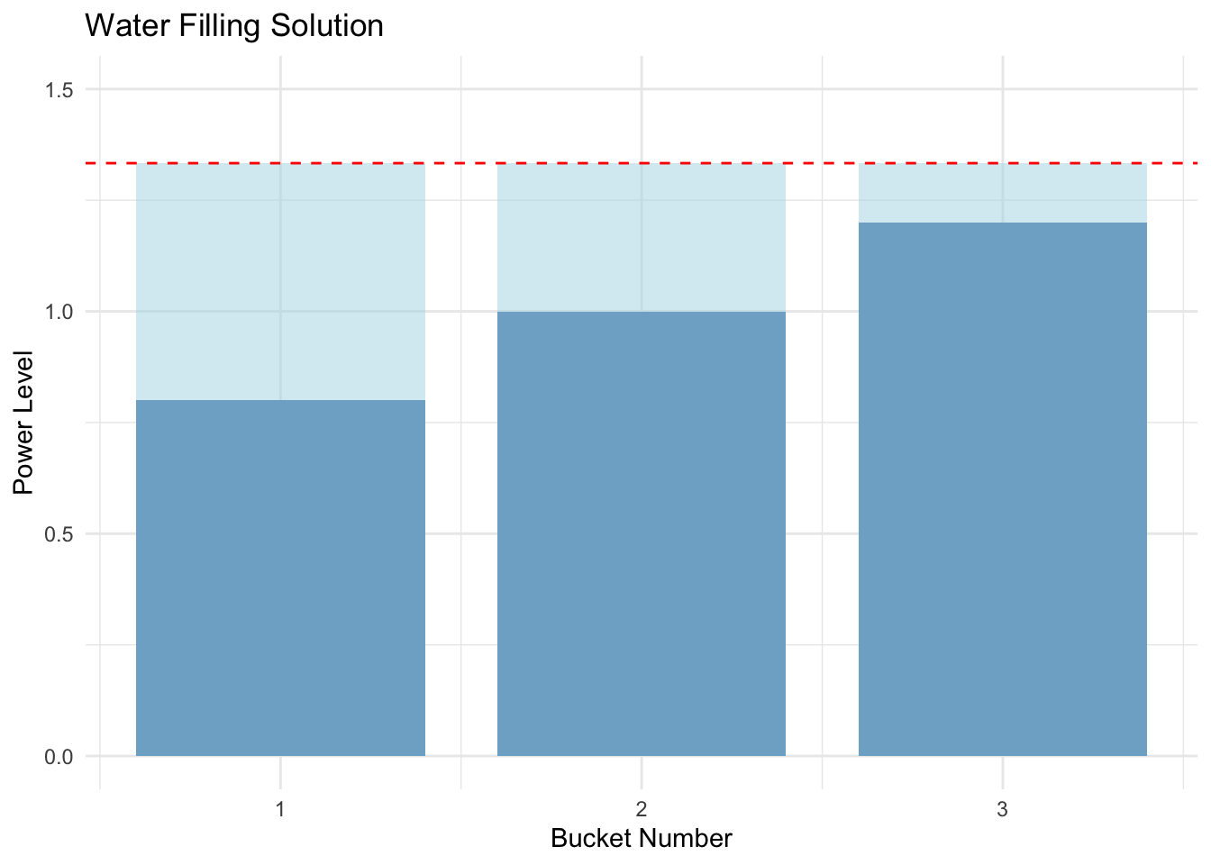
Larger Example
We now solve a larger water filling problem with \(N = 6\) channels and varying floor levels.
n_large <- 6
alpha_large <- c(0.2, 0.5, 0.8, 1.0, 1.2, 1.5)
P_large <- 2

sol_large <- water_filling(n_large, alpha_large, sum_x = P_large)
cat("Problem status:", sol_large$status, "\n")
cat(sprintf("Optimal communication rate = %.4g\n", sol_large$value))
cat("Transmitter powers:\n")
print(round(sol_large$x, 3))
Problem status: optimal
Optimal communication rate = 1.059
Transmitter powers:
[1] 0.925 0.625 0.325 0.125 0.000 0.000x_vals_l <- sol_large$x
y_vals_l <- alpha_large + x_vals_l
df_l <- data.frame(
bucket = seq_len(n_large),
alpha = alpha_large,
total = y_vals_l,
power = x_vals_l
)
ggplot(df_l) +
geom_col(aes(x = bucket, y = alpha), fill = "steelblue", width = 0.8) +
geom_col(aes(x = bucket, y = total), fill = "lightblue", alpha = 0.5, width = 0.8) +
geom_hline(yintercept = max(y_vals_l), linetype = "dashed", color = "red") +
scale_x_continuous(breaks = seq_len(n_large)) +
labs(x = "Bucket Number", y = "Power Level",
title = "Water Filling Solution (6 Channels)") +
theme_minimal()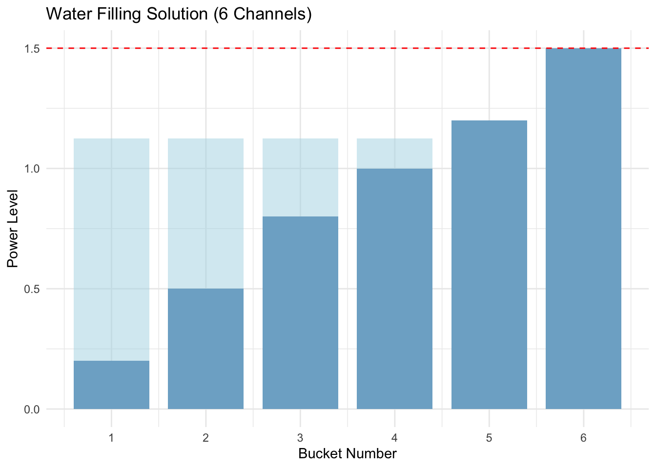
Session Info
R version 4.6.0 (2026-04-24)
Platform: aarch64-apple-darwin23
Running under: macOS Tahoe 26.5.1

Matrix products: default
BLAS:   /Library/Frameworks/R.framework/Versions/4.6/Resources/lib/libRblas.0.dylib
LAPACK: /Library/Frameworks/R.framework/Versions/4.6/Resources/lib/libRlapack.dylib;  LAPACK version 3.12.1

locale:
[1] en_US.UTF-8/en_US.UTF-8/en_US.UTF-8/C/en_US.UTF-8/en_US.UTF-8

time zone: America/Los_Angeles
tzcode source: internal

attached base packages:
[1] stats     graphics  grDevices utils     datasets  methods   base

other attached packages:
[1] ggplot2_4.0.3 CVXR_1.9.1

loaded via a namespace (and not attached):
 [1] piqp_0.6.2         Matrix_1.7-5       gtable_0.3.6       jsonlite_2.0.0
 [5] dplyr_1.2.1        compiler_4.6.0     highs_1.14.0-2     tidyselect_1.2.1
 [9] Rcpp_1.1.1-1.1     slam_0.1-55        cccp_0.3-3         dichromat_2.0-0.1
[13] scales_1.4.0       yaml_2.3.12        fastmap_1.2.0      clarabel_0.11.2
[17] lattice_0.22-9     R6_2.6.1           labeling_0.4.3     generics_0.1.4
[21] knitr_1.51         htmlwidgets_1.6.4  backports_1.5.1    checkmate_2.3.4
[25] tibble_3.3.1       osqp_1.0.0         pillar_1.11.1      RColorBrewer_1.1-3
[29] rlang_1.2.0        xfun_0.58          S7_0.2.2           otel_0.2.0
[33] cli_3.6.6          withr_3.0.2        magrittr_2.0.5     Rglpk_0.6-5.1
[37] digest_0.6.39      grid_4.6.0         gmp_0.7-5.1        lifecycle_1.0.5
[41] ECOSolveR_0.6.1    scs_3.2.7          vctrs_0.7.3        evaluate_1.0.5
[45] glue_1.8.1         farver_2.1.2       codetools_0.2-20   rmarkdown_2.31
[49] pkgconfig_2.0.3    tools_4.6.0        htmltools_0.5.9