Parameters are symbolic representations of constants. Using parameters lets you modify the values of constants without reconstructing the entire problem. When your parametrized problem is constructed according to Disciplined Parametrized Programming (DPP), solving it repeatedly for different values of the parameters can be much faster than repeatedly solving a new problem.
You should read this tutorial if you intend to solve a DCP or DGP problem many times, for different values of the numerical data, or if you want to differentiate through the solution map of a DCP or DGP problem.
What is DPP?
DPP is a ruleset for producing parametrized DCP- or DGP-compliant problems that CVXR can re-canonicalize very quickly. The first time a DPP-compliant problem is solved, CVXR compiles it and caches the mapping from parameters to problem data. As a result, subsequent rewritings of DPP problems can be substantially faster. CVXR allows you to solve parametrized problems that are not DPP, but you will not see a speed-up when doing so.
The DPP Ruleset
DPP places mild restrictions on how parameters can enter expressions in DCP and DGP problems.
DPP for DCP Problems
In DPP, an expression is said to be parameter-affine if it does not involve variables and is affine in its parameters, and it is parameter-free if it does not have parameters. DPP introduces two restrictions to DCP:
Under DPP, all parameters are classified as affine, just like variables.
Under DPP, the product of two expressions is affine when at least one of the expressions is constant, or when one of the expressions is parameter-affine and the other is parameter-free.
An expression is DPP-compliant if it is DCP-compliant subject to these two restrictions. You can check whether an expression or problem is DPP-compliant by calling is_dpp(). For example:
m <-3n <-2x <-Variable(c(n, 1))F <-Parameter(c(m, n))G <-Parameter(c(m, n))g <-Parameter(c(m, 1))gamma <-Parameter(nonneg =TRUE)objective <-p_norm(( F + G ) %*% x - g) + gamma *p_norm(x)cat("Is DPP?", is_dpp(objective), "\n")
Is DPP? TRUE
We can walk through the DPP analysis to understand why objective is DPP-compliant. The product (F + G) %*% x is affine under DPP, because F + G is parameter-affine and x is parameter-free. The difference (F + G) %*% x - g is affine because the addition atom is affine and both (F + G) %*% x and -g are affine. Likewise gamma * p_norm(x) is affine under DPP because gamma is parameter-affine and p_norm(x) is parameter-free. The final objective is then affine under DPP because addition is affine.
Some expressions are DCP-compliant but not DPP-compliant. For example, DPP forbids taking the product of two parametrized expressions:
Just as it is possible to rewrite non-DCP problems in DCP-compliant ways, it is also possible to re-express non-DPP problems in DPP-compliant ways. For example, the above problem can be equivalently written as:
In other cases, you can represent non-DPP transformations of parameters by doing them outside of the DSL, e.g., in R. For example, if P is a parameter and x is a variable, quad_form(x, P) is not DPP. You can represent a parametric quadratic form like so:
As another example, the quotient expr / p is not DPP-compliant when p is a parameter, but this can be rewritten as expr * p_tilde, where p_tilde is a parameter that represents 1/p.
DPP for DGP Problems
Just as DGP is the log-log analogue of DCP, DPP for DGP is the log-log analog of DPP for DCP. DPP introduces two restrictions to DGP:
Under DPP, all positive parameters are classified as log-log-affine, just like positive variables.
Under DPP, the power atom power(x, p) (with base x and exponent p) is log-log affine as long as x and p are not both parametrized.
Note that for powers, the exponent p must be either a numerical constant or a parameter; attempting to construct a power atom in which the exponent is a compound expression will result in an error.
If a parameter appears in a DGP problem as an exponent, it can have any sign. If a parameter appears elsewhere in a DGP problem, it must be positive, i.e., it must be constructed with Parameter(pos = TRUE).
For example, consider the monomial c * power(x, a) * power(y, b) where c is a positive parameter and a, b are parameters. The expressions power(x, a) and power(y, b) are log-log affine, since x and y do not contain parameters. The parameter c is log-log affine because it is positive, and the monomial expression is log-log affine because the product of log-log affine expressions is also log-log affine. This makes the expression DPP-compliant.
Some expressions are DGP-compliant but not DPP-compliant. For example, DPP forbids raising a parametrized expression to a power: power(power(x, a), a) is DGP but not DPP because both the base (power(x, a)) and the exponent (a) involve the same parameter.
You can represent non-DPP transformations of parameters by doing them outside of CVXR, e.g., in R. For example, if a_val <- 2.0, you could precompute b <- Parameter(value = a_val^2) and write power(x, b) instead.
Repeatedly Solving a DPP Problem
The following example demonstrates how parameters can speed up repeated solves of a DPP-compliant DCP problem. We set up a regularized least-squares problem with \(500\) observations and \(200\) variables, and solve it for \(50\) values of the regularization parameter.
n <-500m <-200set.seed(1)A <-matrix(rnorm(n * m), n, m)b <-rnorm(n)## gamma must be nonneg due to DCP rulesgamma <-Parameter(nonneg =TRUE)x <-Variable(m)error <-sum_squares(A %*% x - b)obj <-Minimize(error + gamma *p_norm(x, 1))problem <-Problem(obj)cat("Is DPP?", is_dpp(problem), "\n")
Is DPP? TRUE
We compare two approaches: (1) DPP re-solve, which updates the parameter value and re-solves the same problem object (re-using the cached compilation), and (2) new problem, which constructs a fresh problem with a numeric regularization weight each time (triggering full re-compilation).
gamma_vals <-10^seq(-4, 1, length.out =50)dpp_times <-numeric(length(gamma_vals))new_problem_times <-numeric(length(gamma_vals))for (i inseq_along(gamma_vals)) {## DPP re-solve: update parameter, re-use cached compilationvalue(gamma) <- gamma_vals[i] t1 <-proc.time() result <-psolve(problem)check_solver_status(problem) t2 <-proc.time() dpp_times[i] <- (t2 - t1)["elapsed"]## New problem: construct fresh objective with numeric value obj_new <-Minimize(error + gamma_vals[i] *p_norm(x, 1)) new_prob <-Problem(obj_new) t3 <-proc.time() new_result <-psolve(new_prob)check_solver_status(new_prob) t4 <-proc.time() new_problem_times[i] <- (t4 - t3)["elapsed"]}
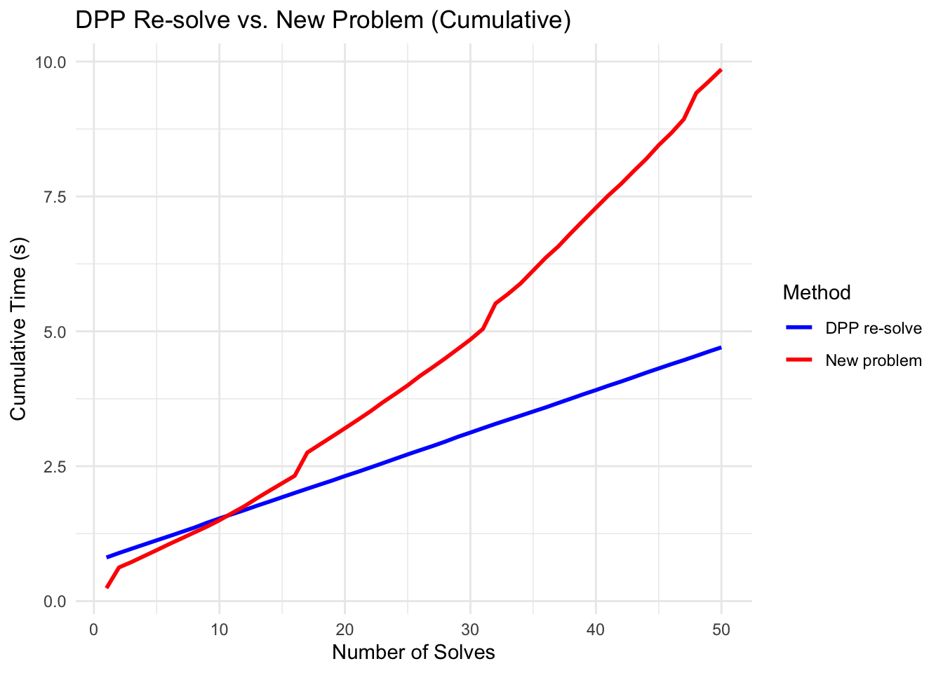
The first DPP solve is slower because it includes the one-time cost of compiling the problem and caching the parameter-to-data mapping. Subsequent DPP solves are faster because they skip re-compilation.
DPP first solve: 0.587 s
DPP subsequent (mean): 0.108 s
New problem (mean): 0.122 s
Per-solve speedup (after first): 1.1x
The cumulative time plot shows the advantage more clearly: the gap widens with each additional solve, demonstrating that the up-front compilation cost is quickly amortized.
df_times <-data.frame(Solve =seq_along(gamma_vals),`DPP re-solve`=cumsum(dpp_times),`New problem`=cumsum(new_problem_times),check.names =FALSE) |>pivot_longer(-Solve, names_to ="Method", values_to ="Time")ggplot(df_times, aes(x = Solve, y = Time, color = Method)) +geom_line(linewidth =1) +scale_color_manual(values =c("DPP re-solve"="blue","New problem"="red")) +labs(x ="Number of Solves", y ="Cumulative Time (s)",title ="DPP Re-solve vs. New Problem (Cumulative)") +theme_minimal()
Agrawal, A., Barratt, S., Boyd, S., Busseti, E., Moursi, W. M. (2019). Differentiating through a cone program. Journal of Applied and Numerical Optimization, 1(2), 107–115.
Agrawal, A., Verschueren, R., Diamond, S., Boyd, S. (2018). A rewriting system for convex optimization problems. Journal of Control and Decision, 5(1), 42–60.