y1 <- Variable(2)
y2 <- Variable(1, integer = TRUE)
y3 <- Variable(1)
x <- vstack(y1, y2, y3) ## Create x expression
C <- matrix(c(1, 2, -0.1, -3), nrow = 1)
objective <- Maximize(C %*% x)
constraints <- list(
    x >= 0,
    x[1] + x[2] <= 5,
    2 * x[1] - x[2] >= 0,
    -x[1] + 3 * x[2] >= 0,
    x[3] + x[4] >= 0.5,
    x[3] >= 1.1)
problem <- Problem(objective, constraints)Integer Programming
Consider the following optimization problem.
\[ \begin{array}{ll} \mbox{Maximize} & x_1 + 2x_2 - 0.1x_3 - 3x_4\\ \mbox{subject to} & x_1, x_2, x_3, x_4 >= 0\\ & x_1 + x_2 <= 5\\ & 2x_1 - x_2 >= 0\\ & -x_1 + 3x_2 >= 0\\ & x_3 + x_4 >= 0.5\\ & x_3 >= 1.1\\ & x_3 \mbox{ is integer.} \end{array} \]
CVXR provides constructors for the integer and boolean variables via the parameter integer = TRUE or boolean = TRUE to the Variable() function. These can be combined with vstack (analog of rbind) or hstack (analog of cbind) to construct new expressions.
The above problem now in CVXR.
We can solve this problem as usual using the HiGHS solver and obtain the optimal value as well as the solution.
## psolve() returns the optimal value; value(x) extracts the solution
## (The deprecated solve()$getValue() pattern still works but warns.)
result <- psolve(problem, solver = "HIGHS")
check_solver_status(problem)
cat(sprintf("Optimal value: %.3f\n", result))
Optimal value: 8.133highs_solution <- value(x)Alternative Solvers
We can try other solvers and compare the solutions obtained. CVXR supports several solvers for integer programs, including HiGHS.
solutions <- data.frame(HiGHS = highs_solution)
row.names(solutions) <- c("$x_1$", "$x_2$", "$x_3$", "$x_4$")
knitr::kable(solutions, format = "html") |>
    kable_styling("striped") |>
column_spec(1:2, background = "#ececec")| HiGHS | |
|---|---|
| $x_1$ | 1.666667 |
| $x_2$ | 3.333333 |
| $x_3$ | 2.000000 |
| $x_4$ | 0.000000 |
Office Assignment Problem
For a slightly more involved example, we consider the office assignment problem.
The goal is to assign six people, Marcelo, Rakesh, Peter, Tom, Marjorie, and Mary Ann, to seven offices. Each office can have no more than one person, and each person gets exactly one office. So there will be one empty office. People can give preferences for the offices, and their preferences are considered based on their seniority. Some offices have windows, some do not, and one window is smaller than others. Additionally, Peter and Tom often work together, so should be in adjacent offices. Marcelo and Rakesh often work together, and should be in adjacent offices.
draw_office_layout()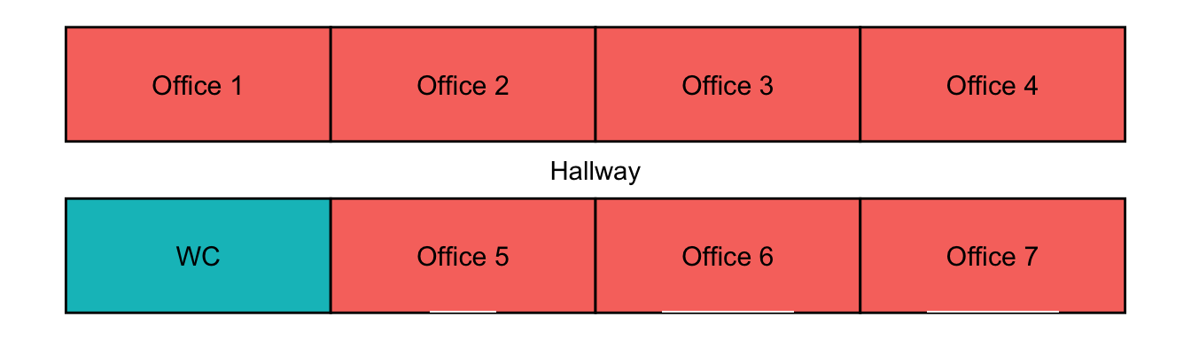
The office layout is shown above. Offices 1, 2, 3, and 4 are inside offices (no windows). Offices 5, 6, and 7 have windows, but the window in office 5 is smaller than the other two.
We begin by recording the names of the people and offices.
people <- c('Mary Ann', 'Marjorie', 'Tom',
            'Peter', 'Marcelo', 'Rakesh')
offices <- c('Office 1', 'Office 2', 'Office 3',
             'Office 4','Office 5', 'Office 6', 'Office 7')
We also have the office preferences of each person for each of the seven offices along with seniority data which is used to scale the office preferences.
preference_matrix <- matrix( c(0, 0, 0, 0, 10, 40, 50,
                               0, 0, 0, 0, 20, 40, 40,
                               0, 0, 0, 0, 30, 40, 30,
                               1, 3, 3, 3, 10, 40, 40,
                               3, 4, 1, 2, 10, 40, 40,
                               10, 10, 10, 10, 20, 20, 20),
                            byrow = TRUE, nrow = length(people))
rownames(preference_matrix) <- people
colnames(preference_matrix) <- offices

seniority <- c(9, 10, 5, 3, 1.5, 2)
weightvector <- seniority / sum(seniority)
PM <- diag(weightvector) %*% preference_matrix
We define the the occupancy variable which indicates, using values 1 or 0, who occupies which office.
occupy <- Variable(c(length(people), length(offices)), integer = TRUE)The objective is to maximize the satisfaction of the preferences weighted by seniority constrained by the fact the a person can only occupy a single office and no office can have more than 1 person.
objective <- Maximize(sum_entries(PM * occupy))

constraints <- list(
    occupy >= 0,
    occupy <= 1,
    sum_entries(occupy, axis = 1) == 1,
    sum_entries(occupy, axis = 2) <= 1
)
We further add the constraint that Tom (person 3) and Peter (person 4) should be no more than one office away, and ditto for Marcelo (person 5) and Rakesh (person 6).
tom_peter <- list(
    occupy[3, 1] + sum_entries(occupy[4, ]) - occupy[4, 2] <= 1,
    occupy[3, 2] + sum_entries(occupy[4, ]) - occupy[4, 1] - occupy[4, 3] - occupy[4, 5] <= 1,
    occupy[3, 3] + sum_entries(occupy[4, ]) - occupy[4, 2] - occupy[4, 4] - occupy[4, 6] <= 1,
    occupy[3, 4] + sum_entries(occupy[4, ]) - occupy[4, 3] - occupy[4, 7] <= 1,
    occupy[3, 5] + sum_entries(occupy[4, ]) - occupy[4, 2] - occupy[4, 6] <= 1,
    occupy[3, 6] + sum_entries(occupy[4, ]) - occupy[4, 3] - occupy[4, 5] - occupy[4, 7] <= 1,
    occupy[3, 7] + sum_entries(occupy[4, ]) - occupy[4, 4] - occupy[4, 6] <= 1
)

marcelo_rakesh <- list(
    occupy[5, 1] + sum_entries(occupy[6, ]) - occupy[6, 2] <= 1,
    occupy[5, 2] + sum_entries(occupy[6, ]) - occupy[6, 1] - occupy[6, 3] - occupy[6, 5] <= 1,
    occupy[5, 3] + sum_entries(occupy[6, ]) - occupy[6, 2] - occupy[6, 4] - occupy[6, 6] <= 1,
    occupy[5, 4] + sum_entries(occupy[6, ]) - occupy[6, 3] - occupy[6, 7] <= 1,
    occupy[5, 5] + sum_entries(occupy[6, ]) - occupy[6, 2] - occupy[6, 6] <= 1,
    occupy[5, 6] + sum_entries(occupy[6, ]) - occupy[6, 3] - occupy[6, 5] - occupy[6, 7] <= 1,
    occupy[5, 7] + sum_entries(occupy[6, ]) - occupy[6, 4] - occupy[6, 6] <= 1
)

constraints <- c(constraints, tom_peter, marcelo_rakesh)
We are now ready to solve the problem.
problem <- Problem(objective, constraints)
ecos_result <- psolve(problem, solver = "HIGHS")
check_solver_status(problem)
ecos_soln <- round(value(occupy), 0)
rownames(ecos_soln) <- people
colnames(ecos_soln) <- offices
We are now ready to plot the solution (after accounting for the WC).
office_assignment <- apply(ecos_soln, 1, which.max)
office_occupants <- names(office_assignment)[match(c(5:7, 1:4), office_assignment)]
office_occupants[is.na(office_occupants)] <- "Empty"
draw_office_layout(c("WC", office_occupants))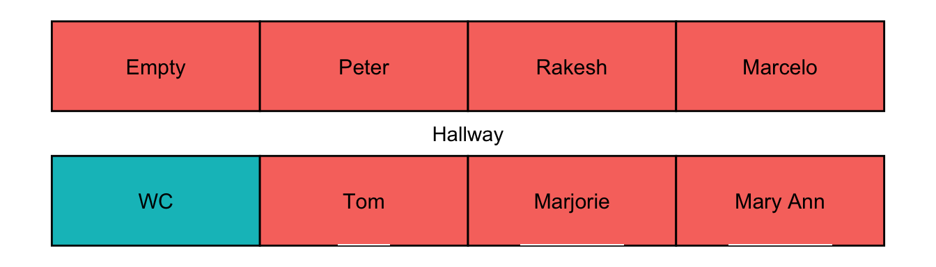
Session Info
R version 4.6.0 (2026-04-24)
Platform: aarch64-apple-darwin23
Running under: macOS Tahoe 26.5.1

Matrix products: default
BLAS:   /Library/Frameworks/R.framework/Versions/4.6/Resources/lib/libRblas.0.dylib
LAPACK: /Library/Frameworks/R.framework/Versions/4.6/Resources/lib/libRlapack.dylib;  LAPACK version 3.12.1

locale:
[1] en_US.UTF-8/en_US.UTF-8/en_US.UTF-8/C/en_US.UTF-8/en_US.UTF-8

time zone: America/Los_Angeles
tzcode source: internal

attached base packages:
[1] stats     graphics  grDevices utils     datasets  methods   base

other attached packages:
[1] ggplot2_4.0.3    kableExtra_1.4.0 CVXR_1.9.1

loaded via a namespace (and not attached):
 [1] gmp_0.7-5.1        generics_0.1.4     clarabel_0.11.2    xml2_1.5.2
 [5] stringi_1.8.7      lattice_0.22-9     digest_0.6.39      magrittr_2.0.5
 [9] evaluate_1.0.5     grid_4.6.0         RColorBrewer_1.1-3 fastmap_1.2.0
[13] rprojroot_2.1.1    jsonlite_2.0.0     Matrix_1.7-5       backports_1.5.1
[17] scs_3.2.7          viridisLite_0.4.3  scales_1.4.0       textshaping_1.0.5
[21] cli_3.6.6          rlang_1.2.0        withr_3.0.2        yaml_2.3.12
[25] otel_0.2.0         tools_4.6.0        osqp_1.0.0         checkmate_2.3.4
[29] dplyr_1.2.1        here_1.0.2         vctrs_0.7.3        R6_2.6.1
[33] lifecycle_1.0.5    stringr_1.6.0      htmlwidgets_1.6.4  pkgconfig_2.0.3
[37] pillar_1.11.1      gtable_0.3.6       glue_1.8.1         Rcpp_1.1.1-1.1
[41] systemfonts_1.3.2  xfun_0.58          tibble_3.3.1       tidyselect_1.2.1
[45] rstudioapi_0.18.0  knitr_1.51         dichromat_2.0-0.1  highs_1.14.0-2
[49] farver_2.1.2       htmltools_0.5.9    labeling_0.4.3     rmarkdown_2.31
[53] svglite_2.2.2      compiler_4.6.0     S7_0.2.2