set.seed(1)

## Problem dimensions
n <- 10        # variable dimension
m <- 400       # total measurements
N <- 4         # number of blocks
block_size <- m / N

## Generate problem data
A_full <- matrix(rnorm(m * n), nrow = m, ncol = n)
x_true <- rnorm(n)
b_full <- A_full %*% x_true + 0.1 * rnorm(m)

## Split data into N blocks
A_blocks <- lapply(1:N, function(i) {
    rows <- ((i-1) * block_size + 1):(i * block_size)
    A_full[rows, ]
})
b_blocks <- lapply(1:N, function(i) {
    rows <- ((i-1) * block_size + 1):(i * block_size)
    b_full[rows]
})Consensus Optimization
Introduction
This example is adapted from the CVXPY documentation on consensus optimization.
Suppose we have a convex optimization problem with \(N\) terms in the objective:
\[ \begin{array}{ll} \mbox{minimize} & \sum_{i=1}^N f_i(x). \end{array} \]
For example, we might be fitting a model to data and \(f_i\) is the loss function for the \(i\)th block of training data.
We can convert this problem into consensus form:
\[ \begin{array}{ll} \mbox{minimize} & \sum_{i=1}^N f_i(x_i) \\ \mbox{subject to} & x_i = z, \end{array} \]
where we interpret the \(x_i\) as local variables (particular to a given \(f_i\)) and \(z\) as the global variable. The constraints \(x_i = z\) enforce consistency, or consensus.
ADMM Algorithm
We can solve a problem in consensus form using the Alternating Direction Method of Multipliers (ADMM). Each iteration of ADMM reduces to the following updates:
\[ \begin{array}{lll} x^{k+1}_i & := & \arg\min_{x_i} \left( f_i(x_i) + \frac{\rho}{2} \left\| x_i - \bar{x}^k + u^k_i \right\|^2_2 \right) \\ u^{k+1}_i & := & u^{k}_i + x^{k+1}_i - \bar{x}^{k+1} \end{array} \]
where \(\bar{x}^k = \frac{1}{N} \sum_{i=1}^N x^k_i\).
Example: Consensus Least Squares
We illustrate the consensus ADMM approach on a simple least-squares problem where the data is split across \(N\) blocks. The original problem is:
\[ \mbox{minimize} \quad \|A x - b\|_2^2, \]
where \(A \in \mathbb{R}^{m \times n}\) and \(b \in \mathbb{R}^m\).
We split \(A\) and \(b\) into \(N\) blocks row-wise, so \(f_i(x) = \|A_i x - b_i\|_2^2\).
Centralized Solution
First, we solve the problem in the standard (non-distributed) way for comparison.
x_central <- Variable(n)
obj_central <- Minimize(sum_squares(A_full %*% x_central - b_full))
prob_central <- Problem(obj_central)
result_central <- psolve(prob_central)

x_central_val <- as.numeric(value(x_central))
cat(sprintf("Centralized solution status: %s\n", status(prob_central)))
cat(sprintf("Centralized objective: %.6f\n", result_central))
Centralized solution status: optimal
Centralized objective: 3.806978ADMM Consensus Solution
Now we implement the consensus ADMM algorithm. In each iteration, we solve \(N\) local subproblems using CVXR and then average to get the global update.
rho <- 1.0
MAX_ITER <- 50

## Initialize
x_vars <- matrix(0, nrow = n, ncol = N)   # local variables
u_vars <- matrix(0, nrow = n, ncol = N)   # dual variables
xbar <- rep(0, n)                          # global average

## Track convergence
obj_history <- numeric(MAX_ITER)

for (iter in seq_len(MAX_ITER)) {
    ## x-update: solve each local subproblem
    for (i in 1:N) {
        x_i <- Variable(n)
        f_i <- sum_squares(A_blocks[[i]] %*% x_i - b_blocks[[i]])
        augmented <- f_i + (rho / 2) * sum_squares(x_i - xbar + u_vars[, i])
        prob_i <- Problem(Minimize(augmented))
        result_i <- psolve(prob_i)
        x_vars[, i] <- as.numeric(value(x_i))
    }

    ## z-update: average the x_i
    xbar <- rowMeans(x_vars)

    ## u-update: update dual variables
    for (i in 1:N) {
        u_vars[, i] <- u_vars[, i] + x_vars[, i] - xbar
    }

    ## Compute objective at current average
    obj_history[iter] <- sum((A_full %*% xbar - b_full)^2)
}

cat(sprintf("ADMM objective after %d iterations: %.6f\n", MAX_ITER, obj_history[MAX_ITER]))
cat(sprintf("Centralized objective: %.6f\n", result_central))
ADMM objective after 50 iterations: 3.815041
Centralized objective: 3.806978Convergence Plot
df_conv <- data.frame(
    iteration = 1:MAX_ITER,
    objective = obj_history
)

ggplot(df_conv, aes(x = iteration, y = objective)) +
    geom_line(color = "steelblue") +
    geom_hline(yintercept = result_central, linetype = "dashed",
               color = "red") +
    annotate("text", x = MAX_ITER * 0.7, y = result_central * 1.05,
             label = "Centralized optimum", color = "red") +
    labs(x = "Iteration", y = "Objective Value",
         title = "ADMM Consensus Convergence") +
    theme_minimal()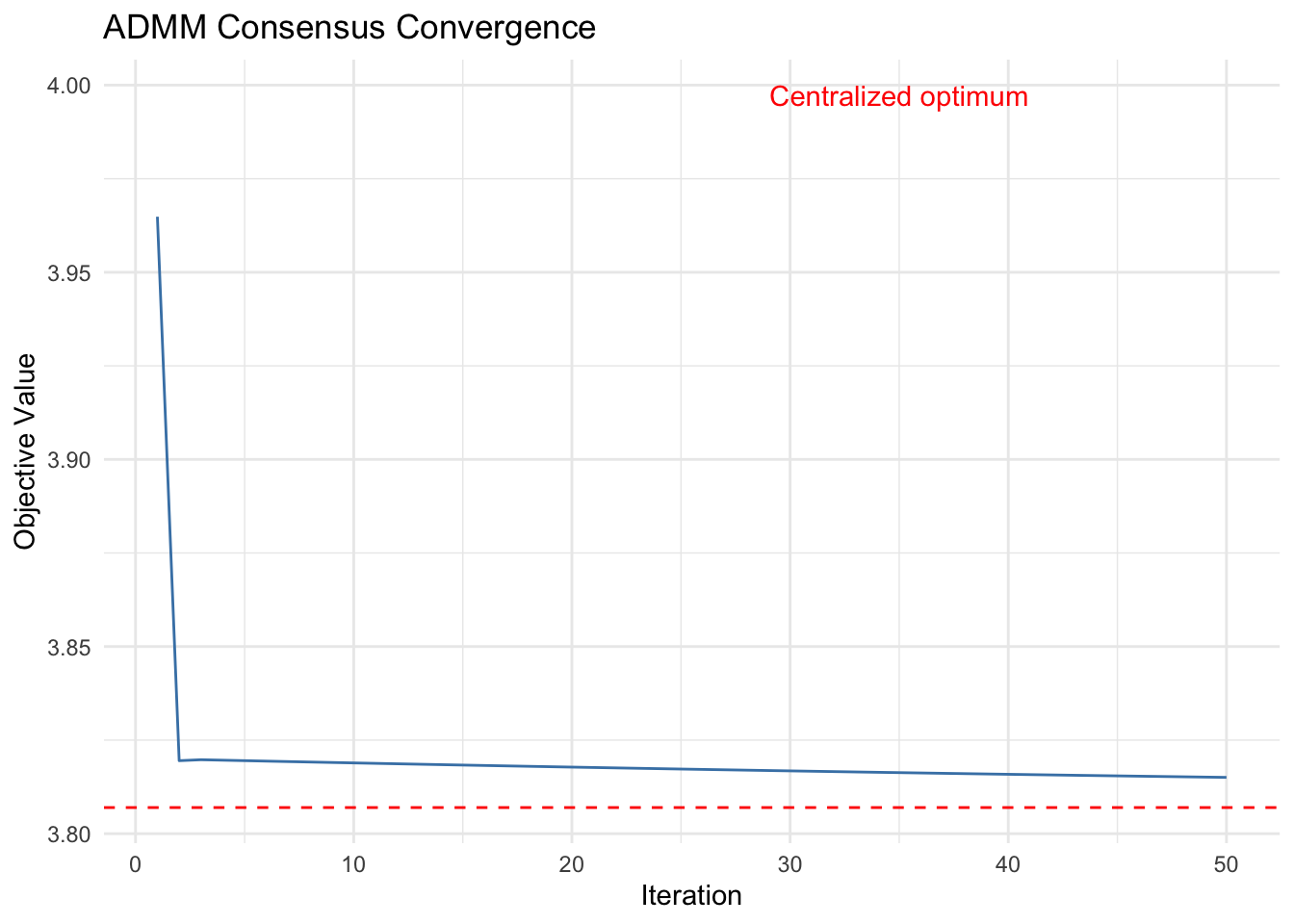
The ADMM consensus solution converges to match the centralized optimal solution.
Comparison of Solutions
cat("Max absolute difference between ADMM and centralized solution:\n")
cat(sprintf("  %.6e\n", max(abs(xbar - x_central_val))))
Max absolute difference between ADMM and centralized solution:
2.464990e-03Session Info
R version 4.6.0 (2026-04-24)
Platform: aarch64-apple-darwin23
Running under: macOS Tahoe 26.5.1

Matrix products: default
BLAS:   /Library/Frameworks/R.framework/Versions/4.6/Resources/lib/libRblas.0.dylib
LAPACK: /Library/Frameworks/R.framework/Versions/4.6/Resources/lib/libRlapack.dylib;  LAPACK version 3.12.1

locale:
[1] en_US.UTF-8/en_US.UTF-8/en_US.UTF-8/C/en_US.UTF-8/en_US.UTF-8

time zone: America/Los_Angeles
tzcode source: internal

attached base packages:
[1] stats     graphics  grDevices utils     datasets  methods   base

other attached packages:
[1] ggplot2_4.0.3 CVXR_1.9.1

loaded via a namespace (and not attached):
 [1] piqp_0.6.2         Matrix_1.7-5       gtable_0.3.6       jsonlite_2.0.0
 [5] dplyr_1.2.1        compiler_4.6.0     highs_1.14.0-2     tidyselect_1.2.1
 [9] Rcpp_1.1.1-1.1     slam_0.1-55        cccp_0.3-3         dichromat_2.0-0.1
[13] scales_1.4.0       yaml_2.3.12        fastmap_1.2.0      clarabel_0.11.2
[17] lattice_0.22-9     R6_2.6.1           labeling_0.4.3     generics_0.1.4
[21] knitr_1.51         htmlwidgets_1.6.4  backports_1.5.1    checkmate_2.3.4
[25] tibble_3.3.1       osqp_1.0.0         pillar_1.11.1      RColorBrewer_1.1-3
[29] rlang_1.2.0        xfun_0.58          S7_0.2.2           otel_0.2.0
[33] cli_3.6.6          withr_3.0.2        magrittr_2.0.5     Rglpk_0.6-5.1
[37] digest_0.6.39      grid_4.6.0         gmp_0.7-5.1        lifecycle_1.0.5
[41] ECOSolveR_0.6.1    scs_3.2.7          vctrs_0.7.3        evaluate_1.0.5
[45] glue_1.8.1         farver_2.1.2       codetools_0.2-20   rmarkdown_2.31
[49] pkgconfig_2.0.3    tools_4.6.0        htmltools_0.5.9
References
- Boyd, S., Parikh, N., Chu, E., Peleato, B. and Eckstein, J. (2011). “Distributed Optimization and Statistical Learning via the Alternating Direction Method of Multipliers.” Foundations and Trends in Machine Learning, 3(1), 1–122.
- Boyd, S. and Vandenberghe, L. (2004). Convex Optimization. Cambridge University Press.