set.seed(1)

n <- 2000
m <- 200
p <- 0.01
snr <- 5

sigma <- sqrt(p * n / (snr^2))
A <- matrix(rnorm(m * n), nrow = m, ncol = n)

x_true <- as.integer(runif(n) <= p)
v <- sigma * rnorm(m)

y <- A %*% x_true + vFault Detection
Introduction
We consider a problem of identifying faults that have occurred in a system based on sensor measurements of system performance. This example is adapted from the CVXPY documentation.
Topic reference: Samar, S., Gorinevsky, D. and Boyd, S. “Likelihood Bounds for Constrained Estimation with Uncertainty.” 44th IEEE Conference on Decision and Control, 2005.
Problem Statement
Each of \(n\) possible faults occurs independently with probability \(p\). The vector \(x \in \{0, 1\}^n\) encodes the fault occurrences, with \(x_i = 1\) indicating that fault \(i\) has occurred. System performance is measured by \(m\) sensors. The sensor output is
\[ y = Ax + v = \sum_{i=1}^n a_i x_i + v, \]
where \(A \in \mathbb{R}^{m \times n}\) is the sensing matrix with column \(a_i\) being the fault signature of fault \(i\), and \(v \in \mathbb{R}^m\) is a noise vector where \(v_j\) is Gaussian with mean 0 and variance \(\sigma^2\).
The objective is to guess \(x\) (which faults have occurred) given \(y\) (sensor measurements).
We are interested in the setting where \(n > m\), that is, when we have more possible faults than measurements. In this setting, we can expect a good recovery when the vector \(x\) is sparse. This is the subject of compressed sensing.
Solution Approach
To identify the faults, one reasonable approach is to choose \(x \in \{0, 1\}^n\) to minimize the negative log-likelihood function
\[ \ell(x) = \frac{1}{2\sigma^2} \|Ax - y\|_2^2 + \log(1/p - 1) \mathbf{1}^T x + c. \]
However, this problem is nonconvex and NP-hard, due to the constraint that \(x\) must be Boolean.
To make this problem tractable, we relax the Boolean constraints and instead constrain \(x_i \in [0, 1]\). The optimization problem
\[ \begin{array}{ll} \mbox{minimize} & \|Ax - y\|_2^2 + 2\sigma^2 \log(1/p - 1) \mathbf{1}^T x \\ \mbox{subject to} & 0 \leq x_i \leq 1, \quad i = 1, \ldots, n \end{array} \]
is convex. We refer to the solution as the relaxed ML estimate.
By rounding the relaxed ML estimate to the nearest of 0 or 1, we recover a Boolean estimate of the fault occurrences.
Example
We generate an example with \(n = 2000\) possible faults, \(m = 200\) measurements, and fault probability \(p = 0.01\). We choose \(\sigma^2\) so that the signal-to-noise ratio is 5, i.e.,
\[ \sqrt{\frac{\mathbf{E}\|Ax\|_2^2}{\mathbf{E}\|v\|_2^2}} = 5. \]
Below, we show the true fault vector \(x\), the signal \(Ax\), and the noise \(v\).
df_x <- data.frame(index = 1:n, value = x_true)
ggplot(df_x, aes(x = index, y = value)) +
    geom_line() +
    labs(x = "Index", y = "x_true", title = "True Faults") +
    theme_minimal()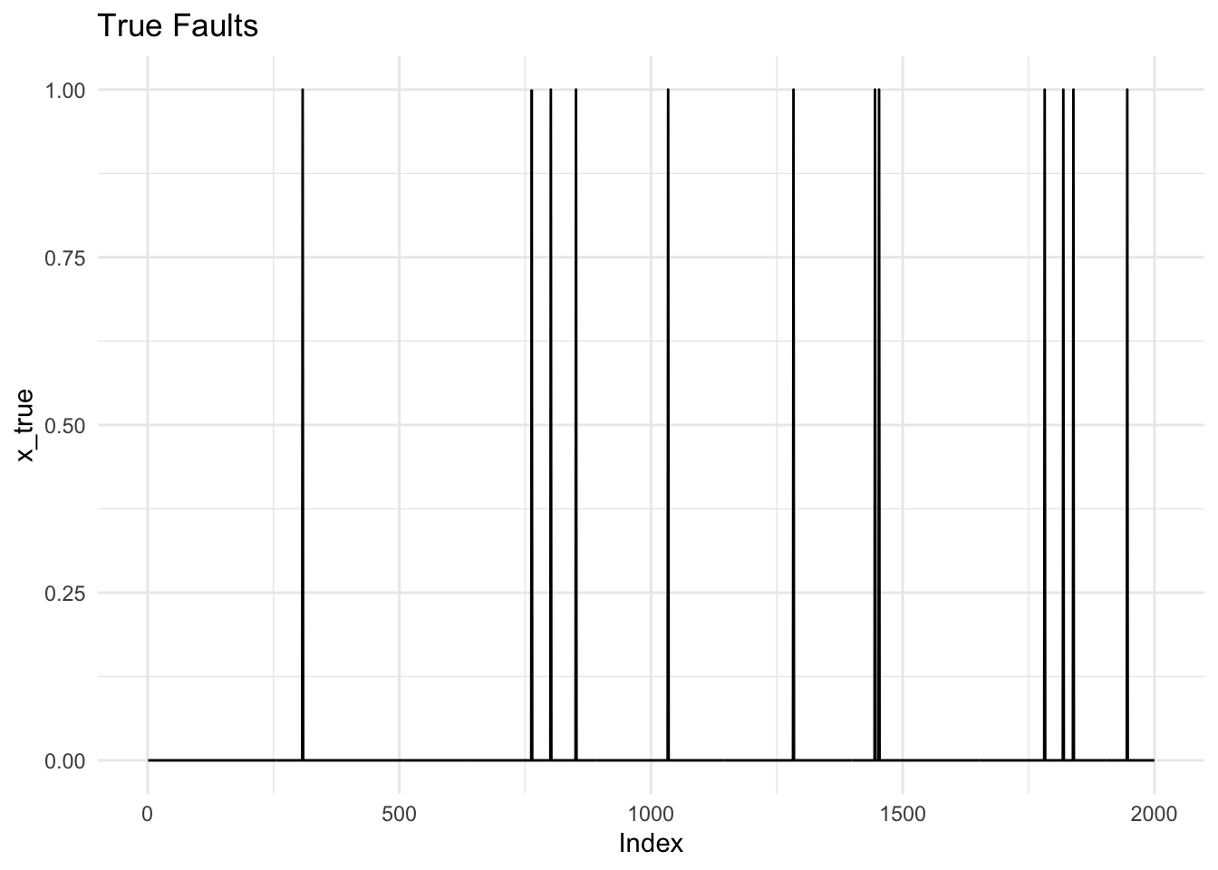
Ax <- as.vector(A %*% x_true)
df_signal <- data.frame(
    index = rep(1:m, 2),
    value = c(Ax, v),
    type = rep(c("Ax", "v"), each = m)
)
ggplot(df_signal, aes(x = index, y = value, color = type)) +
    geom_line() +
    labs(x = "Index", y = "Value", title = "Signal and Noise", color = "") +
    theme_minimal() +
    theme(legend.position = "bottom")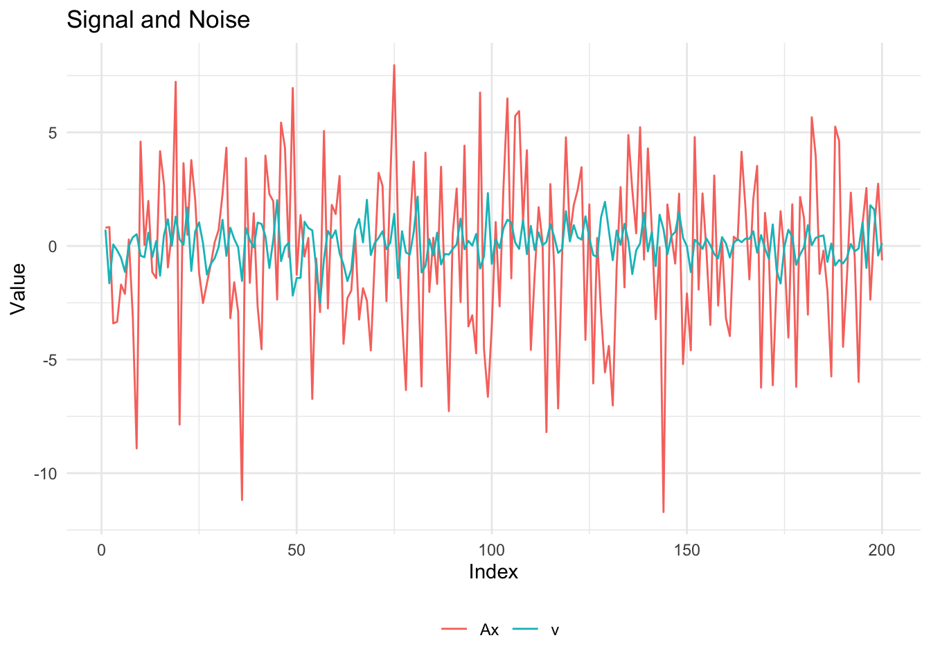
Recovery
We solve the relaxed maximum likelihood problem with CVXR and then round the result to get a Boolean solution.
x_var <- Variable(n)
tau <- 2 * log(1/p - 1) * sigma^2
obj <- Minimize(sum_squares(A %*% x_var - y) + tau * sum(x_var))
constraints <- list(x_var >= 0, x_var <= 1)
prob <- Problem(obj, constraints)
result <- psolve(prob)
Warning: Solution may be inaccurate. Try another solver, adjusting the solver settings,
or solve with `verbose = TRUE` for more information.cat(sprintf("Problem status: %s\n", status(prob)))
cat(sprintf("Final objective value: %.4f\n", result))
## Relaxed ML estimate
x_rml <- as.numeric(value(x_var))
## Rounded solution
x_rnd <- as.integer(x_rml >= 0.5)Problem status: optimal_inaccurate
Final objective value: 126.4516Evaluation
We compute the estimation errors and plot the true, relaxed ML, and rounded solutions.
errors <- function(x_true, x_est, threshold = 0.5) {
    k <- sum(x_true)
    false_pos <- sum(x_true < threshold & x_est >= threshold)
    false_neg <- sum(x_true >= threshold & x_est < threshold)
    list(true_faults = k, false_positives = false_pos, false_negatives = false_neg)
}

err <- errors(x_true, x_rml)
cat(sprintf("True faults: %d\n", err$true_faults))
cat(sprintf("False positives: %d\n", err$false_positives))
cat(sprintf("False negatives: %d\n", err$false_negatives))
True faults: 12
False positives: 0
False negatives: 0df_plot <- data.frame(
index = rep(1:n, 3),
value = c(x_true, x_rml, x_rnd),
type = factor(rep(c("x_true", "x_rml (relaxed ML)", "x_rnd (rounded)"),
each = n),
levels = c("x_true", "x_rml (relaxed ML)", "x_rnd (rounded)"))
)
ggplot(df_plot, aes(x = index, y = value)) +
geom_line() +
facet_wrap(~ type, nrow = 1) +
coord_cartesian(ylim = c(0, 1)) +
labs(x = "Index", y = "Value") +
theme_minimal()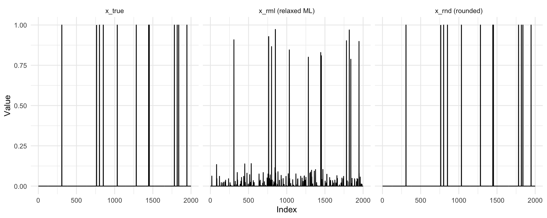
The rounded solution gives perfect recovery with 0 false negatives and 0 false positives.
Session Info
R version 4.6.0 (2026-04-24)
Platform: aarch64-apple-darwin23
Running under: macOS Tahoe 26.5.1

Matrix products: default
BLAS:   /Library/Frameworks/R.framework/Versions/4.6/Resources/lib/libRblas.0.dylib
LAPACK: /Library/Frameworks/R.framework/Versions/4.6/Resources/lib/libRlapack.dylib;  LAPACK version 3.12.1

locale:
[1] en_US.UTF-8/en_US.UTF-8/en_US.UTF-8/C/en_US.UTF-8/en_US.UTF-8

time zone: America/Los_Angeles
tzcode source: internal

attached base packages:
[1] stats     graphics  grDevices utils     datasets  methods   base

other attached packages:
[1] ggplot2_4.0.3 CVXR_1.9.1

loaded via a namespace (and not attached):
 [1] piqp_0.6.2         Matrix_1.7-5       gtable_0.3.6       jsonlite_2.0.0
 [5] dplyr_1.2.1        compiler_4.6.0     highs_1.14.0-2     tidyselect_1.2.1
 [9] Rcpp_1.1.1-1.1     slam_0.1-55        cccp_0.3-3         dichromat_2.0-0.1
[13] scales_1.4.0       yaml_2.3.12        fastmap_1.2.0      clarabel_0.11.2
[17] lattice_0.22-9     R6_2.6.1           labeling_0.4.3     generics_0.1.4
[21] knitr_1.51         htmlwidgets_1.6.4  backports_1.5.1    checkmate_2.3.4
[25] tibble_3.3.1       osqp_1.0.0         pillar_1.11.1      RColorBrewer_1.1-3
[29] rlang_1.2.0        xfun_0.58          S7_0.2.2           otel_0.2.0
[33] cli_3.6.6          withr_3.0.2        magrittr_2.0.5     Rglpk_0.6-5.1
[37] digest_0.6.39      grid_4.6.0         gmp_0.7-5.1        lifecycle_1.0.5
[41] ECOSolveR_0.6.1    scs_3.2.7          vctrs_0.7.3        evaluate_1.0.5
[45] glue_1.8.1         farver_2.1.2       codetools_0.2-20   rmarkdown_2.31
[49] pkgconfig_2.0.3    tools_4.6.0        htmltools_0.5.9
References
- Samar, S., Gorinevsky, D. and Boyd, S. (2005). “Likelihood Bounds for Constrained Estimation with Uncertainty.” 44th IEEE Conference on Decision and Control (CDC-ECC’05), IEEE.