The Catenary Problem

Author

Anqi Fu and Balasubramanian Narasimhan

Introduction

A chain with uniformly distributed mass hangs from the endpoints $(0, 1)$ and $(1, 1)$ on a 2-D plane. Gravitational force acts in the negative $y$ direction. Our goal is to find the shape of the chain in equilibrium, which is equivalent to determining the $(x, y)$ coordinates of every point along its curve when its potential energy is minimized.

This is the famous catenary problem.

A Discrete Version

To formulate as an optimization problem, we parameterize the chain by its arc length and divide it into $m$ discrete links. The length of each link must be no more than $h > 0$ . Since mass is uniform, the total potential energy is simply the sum of the $y$ -coordinates. Therefore, our (discretized) problem is

$\begin{array}{ll} \underset{x, y}{minimize} & \sum_{i = 1}^{m} y_{i} \\ subject to & x_{1} = 0, y_{1} = 1, x_{m} = 1, y_{m} = 1 \\ (x_{i + 1} - x_{i})^{2} + (y_{i + 1} - y_{i})^{2} \leq h^{2}, i = 1, \dots, m - 1 \end{array}$

with variables $x \in R^{m}$ and $y \in R^{m}$ . This discretized version which has been studied by Griva and Vanderbei (2005) was suggested to us by Hans Werner Borchers.

The basic catenary problem has a well-known analytical solution (see Gelfand and Fomin (1963)) which we can easily verify with CVXR.

## Problem data
m <- 101
L <- 2
h <- L / (m - 1)

## Form objective
x <- Variable(m)
y <- Variable(m)
objective <- Minimize(sum(y))

## Form constraints
constraints <- list(x[1] == 0, y[1] == 1,
                    x[m] == 1, y[m] == 1,
                    diff(x)^2 + diff(y)^2 <= h^2)

## Solve the catenary problem
prob <- Problem(objective, constraints)
result <- psolve(prob)
check_solver_status(prob)

We can now plot it and compare it with the ideal solution. Below we use alpha blending and differing line thickness to show the ideal in red and the computed solution in blue.

xs <- value(x)
ys <- value(y)

catenary <- ggplot(data.frame(x = xs, y = ys)) +
    geom_line(mapping = aes(x = x, y = y), color = "blue", linewidth = 1) +
    geom_point(data = data.frame(x = c(xs[1], ys[1]), y = c(xs[m], ys[m])),
               mapping = aes(x = x, y = y), color = "red") 

ideal <- function(x) { 0.22964 *cosh((x -0.5) / 0.22964) - 0.02603 }

catenary + stat_function(fun = ideal , colour = "brown", alpha = 0.5, linewidth = 3)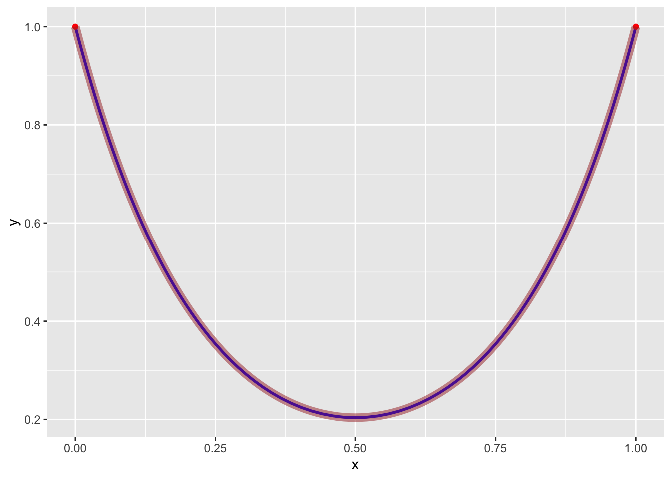

Analytic (red) and computed solution (blue) to the catenary problem

Additional Ground Constraints

A more interesting situation arises when the ground is not flat. Let $g \in R^{m}$ be the elevation vector (relative to the $x$ -axis), and suppose the right endpoint of our chain has been lowered by $Δ y_{m} = 0.5$ . The analytical solution in this case would be difficult to calculate. However, we need only add two lines to our constraint definition,

constr[[4]] <- (y[m] == 0.5)
constr <- c(constr, y >= g)

to obtain the new result.

Below, we define $g$ as a staircase function and solve the problem.

## Lower right endpoint and add staircase structure
ground <- sapply(seq(0, 1, length.out = m), function(x) {
    if(x < 0.2)
        return(0.6)
    else if(x >= 0.2 && x < 0.4)
        return(0.4)
    else if(x >= 0.4 && x < 0.6)
        return(0.2)
    else
        return(0)
})
constraints <- c(constraints, y >= ground)
constraints[[4]] <- (y[m] == 0.5)
prob <- Problem(objective, constraints)
result <- psolve(prob)
check_solver_status(prob)

to obtain the new result.

The figure below shows the solution of this modified catenary problem for $m = 101$ and $h = 0.04$ . The chain is shown hanging in blue, bounded below by the red staircase structure, which represents the ground.

xs <- value(x)
ys <- value(y)

ggplot(data.frame(x = xs, y = ys)) +
    geom_line(mapping = aes(x = x, y = y), color = "blue") +
    geom_point(data = data.frame(x = c(xs[1], ys[1]), y = c(xs[m], ys[m])),
               mapping = aes(x = x, y = y), color = "red") +
    geom_line(data.frame(x = xs, y = ground),
              mapping = aes(x = x, y = y), color = "brown")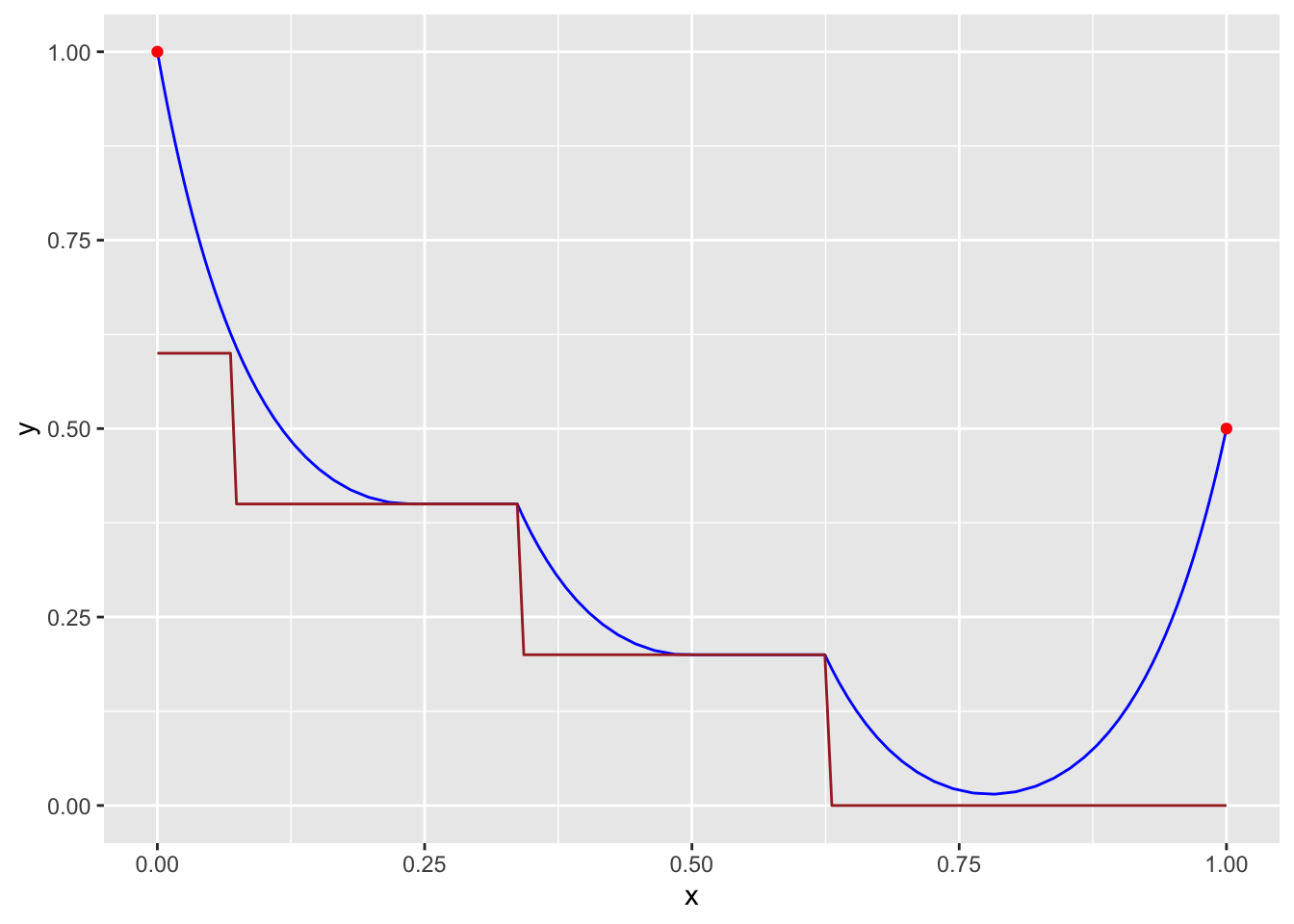

Asymmetric catenary problem with ground constraints.

Session Info

R version 4.5.2 (2025-10-31)
Platform: aarch64-apple-darwin20
Running under: macOS Tahoe 26.3.1

Matrix products: default
BLAS:   /Library/Frameworks/R.framework/Versions/4.5-arm64/Resources/lib/libRblas.0.dylib 
LAPACK: /Library/Frameworks/R.framework/Versions/4.5-arm64/Resources/lib/libRlapack.dylib;  LAPACK version 3.12.1

locale:
[1] en_US.UTF-8/en_US.UTF-8/en_US.UTF-8/C/en_US.UTF-8/en_US.UTF-8

time zone: America/Los_Angeles
tzcode source: internal

attached base packages:
[1] stats     graphics  grDevices utils     datasets  methods   base     

other attached packages:
[1] ggplot2_4.0.2 CVXR_1.8.1   

loaded via a namespace (and not attached):
 [1] gmp_0.7-5.1        generics_0.1.4     clarabel_0.11.2    slam_0.1-55       
 [5] lattice_0.22-9     digest_0.6.39      magrittr_2.0.4     evaluate_1.0.5    
 [9] grid_4.5.2         RColorBrewer_1.1-3 fastmap_1.2.0      rprojroot_2.1.1   
[13] jsonlite_2.0.0     Matrix_1.7-4       ECOSolveR_0.6.1    backports_1.5.0   
[17] scs_3.2.7          Rmosek_11.1.1      scales_1.4.0       codetools_0.2-20  
[21] cli_3.6.5          rlang_1.1.7        Rglpk_0.6-5.1      withr_3.0.2       
[25] yaml_2.3.12        otel_0.2.0         tools_4.5.2        osqp_1.0.0        
[29] Rcplex_0.3-8       checkmate_2.3.4    dplyr_1.2.0        here_1.0.2        
[33] gurobi_13.0-1      vctrs_0.7.1        R6_2.6.1           lifecycle_1.0.5   
[37] htmlwidgets_1.6.4  pkgconfig_2.0.3    cccp_0.3-3         pillar_1.11.1     
[41] gtable_0.3.6       glue_1.8.0         Rcpp_1.1.1         xfun_0.56         
[45] tibble_3.3.1       tidyselect_1.2.1   knitr_1.51         dichromat_2.0-0.1 
[49] highs_1.12.0-3     farver_2.1.2       htmltools_0.5.9    labeling_0.4.3    
[53] rmarkdown_2.30     piqp_0.6.2         compiler_4.5.2     S7_0.2.1

References

Gelfand, I. M., and S. V. Fomin. 1963. Calculus of Variations. Prentice-Hall.

Griva, I. A., and R. J. Vanderbei. 2005. “Case Studies in Optimization: Catenary Problem.” Optimization and Engineering 6 (4): 463–82.