Nonnegative Matrix Factorization

Author

CVXPY Developers and Balasubramanian Narasimhan

Introduction

Adapted from the CVX example of the same name, by Argyris Zymnis, Joelle Skaf, and Stephen Boyd.

We are given a matrix $A \in R^{m \times n}$ and are interested in solving the problem:

$\begin{array}{ll} minimize & ∥ A - Y X ∥_{F} \\ subject to & Y ⪰ 0 \\ X ⪰ 0, \end{array}$

where $Y \in R^{m \times k}$ and $X \in R^{k \times n}$ .

This example generates a random matrix $A$ and obtains an approximate solution to the above problem by first generating a random initial guess for $Y$ and then alternatively minimizing over $X$ and $Y$ for a fixed number of iterations.

Generate Problem Data

## Ensure repeatably random problem data
set.seed(0)

## Generate random data matrix A
m <- 10
n <- 10
k <- 5
A <- matrix(runif(m * k), nrow = m, ncol = k) %*%
     matrix(runif(k * n), nrow = k, ncol = n)

## Initialize Y randomly
Y_init <- matrix(runif(m * k), nrow = m, ncol = k)

Perform Alternating Minimization

We alternate between optimizing over $X$ (with $Y$ fixed) and optimizing over $Y$ (with $X$ fixed). In each sub-problem, the nonnegative variable is optimized while the other factor is held constant as a numeric matrix.

## Ensure same initial random Y
Y_val <- Y_init

MAX_ITERS <- 30
residual <- numeric(MAX_ITERS)

for (iter_num in seq_len(MAX_ITERS)) {
    ## For odd iterations, treat Y constant, optimize over X
    if (iter_num %% 2 == 1) {
        X_var <- Variable(c(k, n))
        constraint <- list(X_var >= 0)
        obj <- Minimize(p_norm(vec(A - Y_val %*% X_var), 2))
        prob <- Problem(obj, constraint)
        result <- psolve(prob, solver = "SCS", max_iters = 10000L)
    } else {
        ## For even iterations, treat X constant, optimize over Y
        Y_var <- Variable(c(m, k))
        constraint <- list(Y_var >= 0)
        obj <- Minimize(p_norm(vec(A - Y_var %*% X_val), 2))
        prob <- Problem(obj, constraint)
        result <- psolve(prob, solver = "SCS", max_iters = 10000L)
    }

    if (!(status(prob) %in% c("optimal", "optimal_inaccurate"))) {
        stop(sprintf("Solver did not converge at iteration %d! Status: %s",
                     iter_num, status(prob)))
    }

    cat(sprintf("Iteration %d, residual norm %.6f\n", iter_num, result))
    residual[iter_num] <- result

    ## Convert variable to numeric for next iteration
    if (iter_num %% 2 == 1) {
        X_val <- value(X_var)
    } else {
        Y_val <- value(Y_var)
    }
}

Iteration 1, residual norm 4.812942
Iteration 2, residual norm 0.391006
Iteration 3, residual norm 0.193455
Iteration 4, residual norm 0.153167
Iteration 5, residual norm 0.124833
Iteration 6, residual norm 0.106494
Iteration 7, residual norm 0.091010
Iteration 8, residual norm 0.079353
Iteration 9, residual norm 0.069269
Iteration 10, residual norm 0.061539
Iteration 11, residual norm 0.054960
Iteration 12, residual norm 0.049648
Iteration 13, residual norm 0.044779
Iteration 14, residual norm 0.040332
Iteration 15, residual norm 0.036093
Iteration 16, residual norm 0.032296
Iteration 17, residual norm 0.028737
Iteration 18, residual norm 0.025548
Iteration 19, residual norm 0.022577
Iteration 20, residual norm 0.019926
Iteration 21, residual norm 0.017487
Iteration 22, residual norm 0.015329
Iteration 23, residual norm 0.013373
Iteration 24, residual norm 0.011653
Iteration 25, residual norm 0.010115
Iteration 26, residual norm 0.008773
Iteration 27, residual norm 0.007581
Iteration 28, residual norm 0.006550
Iteration 29, residual norm 0.005648
Iteration 30, residual norm 0.004865

Output Results

Residual Plot

df_resid <- data.frame(
    iteration = seq_len(MAX_ITERS),
    residual = residual
)

ggplot(df_resid, aes(x = iteration, y = residual)) +
    geom_line() +
    geom_point(size = 1) +
    labs(x = "Iteration Number", y = "Residual Norm",
         title = "Nonnegative Matrix Factorization Convergence") +
    theme_minimal()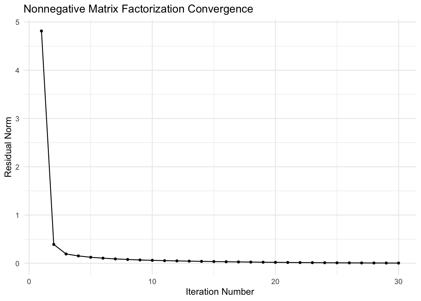

Convergence of alternating minimization for NMF

Factor Matrices

cat("Original matrix A:\n")
print(round(A, 4))

cat("\nLeft factor Y:\n")
print(round(Y_val, 4))

cat("\nRight factor X:\n")
print(round(X_val, 4))

cat("\nResidual A - Y %*% X:\n")
print(round(A - Y_val %*% X_val, 6))

cat(sprintf("\nFinal residual after %d iterations: %.6f\n",
            MAX_ITERS, residual[MAX_ITERS]))

Original matrix A:
        [,1]   [,2]   [,3]   [,4]   [,5]   [,6]   [,7]   [,8]   [,9]  [,10]
 [1,] 1.5700 0.7642 0.9424 1.2671 1.7137 1.6067 1.7121 1.3866 0.7681 1.5747
 [2,] 1.4994 1.1284 1.0647 1.1118 1.5280 1.9443 1.4705 1.1676 1.1715 1.6600
 [3,] 0.9459 0.8503 0.8652 0.9032 0.9875 1.2549 1.0357 0.7002 1.0602 1.2978
 [4,] 1.6941 1.0892 1.5384 1.3061 1.7138 2.2502 1.7654 1.2886 1.2882 2.1279
 [5,] 1.1377 0.6048 1.0263 0.9396 1.2798 1.3864 1.3833 1.0132 0.8338 1.5956
 [6,] 1.2297 0.9551 1.4192 1.1364 1.1255 1.7483 1.2220 0.7295 1.2247 1.6614
 [7,] 1.6787 1.1044 1.5024 1.4767 1.7745 2.0800 1.8787 1.3307 1.3918 2.1866
 [8,] 1.3624 0.5697 1.4157 1.4170 1.3646 1.4297 1.5542 0.9726 0.8387 1.6587
 [9,] 1.4249 0.6382 1.4948 0.9919 1.4324 1.9433 1.5368 1.1035 0.8424 1.9109
[10,] 1.8626 1.2175 1.4339 1.5400 1.9049 2.2419 1.9169 1.4396 1.3390 2.0796

Left factor Y:
        [,1]   [,2]   [,3]   [,4]   [,5]
 [1,] 1.1870 0.9996 0.0095 0.7677 0.0000
 [2,] 1.0810 0.3271 0.5001 0.6120 0.2241
 [3,] 0.0218 0.6801 0.9088 0.0000 0.5639
 [4,] 0.8650 0.4347 0.5539 0.6527 0.7693
 [5,] 0.3821 1.0958 0.4233 0.0827 0.8758
 [6,] 0.0214 0.0000 0.8957 0.4988 0.7037
 [7,] 0.4525 1.1006 0.8651 0.3464 0.8880
 [8,] 0.0000 0.7218 0.4299 0.7361 0.5013
 [9,] 0.8369 0.1929 0.0605 0.7042 0.9551
[10,] 1.0114 0.6444 0.5788 0.8273 0.3190

Right factor X:
       [,1]   [,2]   [,3]   [,4]   [,5]   [,6]   [,7]   [,8]   [,9]  [,10]
[1,] 0.4072 0.4873 0.0000 0.0000 0.4746 0.7149 0.3228 0.4423 0.3621 0.4027
[2,] 0.3443 0.0001 0.1154 0.4496 0.4838 0.0593 0.5480 0.4194 0.0494 0.3366
[3,] 0.5748 0.9154 0.4166 0.5764 0.5159 0.9006 0.4478 0.2954 0.9809 0.6606
[4,] 0.9590 0.2300 1.0724 1.0571 0.8619 0.8987 1.0122 0.5727 0.3649 0.9835
[5,] 0.3221 0.0136 0.7248 0.1318 0.3181 0.6766 0.4408 0.2423 0.2237 0.8129

Residual A - Y %*% X:
           [,1]      [,2]      [,3]      [,4]      [,5]      [,6]      [,7]
 [1,]  0.000704  0.000343 -0.000204  0.000601  0.000117  0.000305 -0.000240
 [2,]  0.000085 -0.000075 -0.000140  0.000036 -0.000050  0.000054  0.000040
 [3,] -0.001172 -0.000051 -0.000661 -0.000704 -0.000033 -0.001006  0.000424
 [4,]  0.000043 -0.000037 -0.000069  0.000018 -0.000025  0.000028  0.000019
 [5,]  0.000020 -0.000013 -0.000025  0.000007 -0.000009  0.000015  0.000006
 [6,]  0.001073  0.000375  0.001038  0.000028 -0.000452  0.001832 -0.001140
 [7,]  0.000005  0.000000 -0.000001  0.000001 -0.000001  0.000006 -0.000002
 [8,] -0.000698 -0.000017  0.000618  0.000474 -0.000237 -0.000970  0.000075
 [9,]  0.000022 -0.000019 -0.000036  0.000009 -0.000013  0.000014  0.000010
[10,]  0.000022 -0.000019 -0.000036  0.000009 -0.000013  0.000014  0.000010
           [,8]      [,9]     [,10]
 [1,] -0.000089 -0.000461 -0.001102
 [2,] -0.000134  0.000005  0.000079
 [3,]  0.000274  0.001158  0.001388
 [4,] -0.000066  0.000001  0.000038
 [5,] -0.000026 -0.000003  0.000010
 [6,] -0.000727 -0.001078 -0.001578
 [7,] -0.000003 -0.000004 -0.000004
 [8,] -0.000177  0.000665  0.000377
 [9,] -0.000034  0.000001  0.000021
[10,] -0.000035  0.000001  0.000020

Final residual after 30 iterations: 0.004865

Session Info

R version 4.5.2 (2025-10-31)
Platform: aarch64-apple-darwin20
Running under: macOS Tahoe 26.3

Matrix products: default
BLAS:   /Library/Frameworks/R.framework/Versions/4.5-arm64/Resources/lib/libRblas.0.dylib 
LAPACK: /Library/Frameworks/R.framework/Versions/4.5-arm64/Resources/lib/libRlapack.dylib;  LAPACK version 3.12.1

locale:
[1] en_US.UTF-8/en_US.UTF-8/en_US.UTF-8/C/en_US.UTF-8/en_US.UTF-8

time zone: America/Los_Angeles
tzcode source: internal

attached base packages:
[1] stats     graphics  grDevices utils     datasets  methods   base     

other attached packages:
[1] ggplot2_4.0.2 CVXR_1.8.1   

loaded via a namespace (and not attached):
 [1] gmp_0.7-5.1        generics_0.1.4     clarabel_0.11.2    slam_0.1-55       
 [5] lattice_0.22-9     digest_0.6.39      magrittr_2.0.4     evaluate_1.0.5    
 [9] grid_4.5.2         RColorBrewer_1.1-3 fastmap_1.2.0      jsonlite_2.0.0    
[13] Matrix_1.7-4       ECOSolveR_0.6.1    backports_1.5.0    scs_3.2.7         
[17] Rmosek_11.1.1      scales_1.4.0       codetools_0.2-20   cli_3.6.5         
[21] rlang_1.1.7        Rglpk_0.6-5.1      withr_3.0.2        yaml_2.3.12       
[25] otel_0.2.0         tools_4.5.2        osqp_1.0.0         Rcplex_0.3-8      
[29] checkmate_2.3.4    dplyr_1.2.0        gurobi_13.0-1      vctrs_0.7.1       
[33] R6_2.6.1           lifecycle_1.0.5    htmlwidgets_1.6.4  pkgconfig_2.0.3   
[37] cccp_0.3-3         pillar_1.11.1      gtable_0.3.6       glue_1.8.0        
[41] Rcpp_1.1.1         xfun_0.56          tibble_3.3.1       tidyselect_1.2.1  
[45] knitr_1.51         dichromat_2.0-0.1  highs_1.12.0-3     farver_2.1.2      
[49] htmltools_0.5.9    rmarkdown_2.30     labeling_0.4.3     piqp_0.6.2        
[53] compiler_4.5.2     S7_0.2.1