set.seed(1)
## Calculate a piecewise linear function
pwl_fun <- function(x, knots) {
    n <- nrow(knots)
    x0 <- sort(knots$x, decreasing = FALSE)
    y0 <- knots$y[order(knots$x, decreasing = FALSE)]
    slope <- diff(y0)/diff(x0)

    sapply(x, function(xs) {
        if(xs <= x0[1])
            y0[1] + slope[1]*(xs -x0[1])
        else if(xs >= x0[n])
            y0[n] + slope[n-1]*(xs - x0[n])
        else {
            idx <- which(xs <= x0)[1]
            y0[idx-1] + slope[idx-1]*(xs - x0[idx-1])
        }
    })
}
## Problem data
m <- 25
xrange <- 0:100
knots <- data.frame(x = c(0, 25, 65, 100), y = c(10, 30, 40, 15))
xprobs <- pwl_fun(xrange, knots)/15
xprobs <- exp(xprobs)/sum(exp(xprobs))
x <- sample(xrange, size = m, replace = TRUE, prob = xprobs)

K <- max(xrange)
counts <- hist(x, breaks = -1:K, right = TRUE, include.lowest = FALSE,
plot = FALSE)$countsLog-Concave Distribution Estimation
Introduction
Let \(n = 1\) and suppose \(x_i\) are i.i.d. samples from a log-concave discrete distribution on \(\{0,\ldots,K\}\) for some \(K \in {\mathbf Z}_+\). Define \(p_k := {\mathbf {Prob}}(X = k)\) to be the probability mass function. One method for estimating \(\{p_0,\ldots,p_K\}\) is to maximize the log-likelihood function subject to a log-concavity constraint , i.e.,
\[ \begin{array}{ll} \underset{p}{\mbox{maximize}} & \sum_{k=0}^K M_k\log p_k \\ \mbox{subject to} & p \geq 0, \quad \sum_{k=0}^K p_k = 1, \\ & p_k \geq \sqrt{p_{k-1}p_{k+1}}, \quad k = 1,\ldots,K-1, \end{array} \]
where \(p \in {\mathbf R}^{K+1}\) is our variable of interest and \(M_k\) represents the number of observations equal to \(k\), so that \(\sum_{k=0}^K M_k = m\). The problem as posed above is not convex. However, we can transform it into a convex optimization problem by defining new variables \(u_k = \log p_k\) and relaxing the equality constraint to \(\sum_{k=0}^K p_k \leq 1\), since the latter always holds tightly at an optimal solution. The result is
\[ \begin{array}{ll} \underset{u}{\mbox{maximize}} & \sum_{k=0}^K M_k u_k \\ \mbox{subject to} & \sum_{k=0}^K e^{u_k} \leq 1, \\ & u_k - u_{k-1} \geq u_{k+1} - u_k, \quad k = 1,\ldots,K-1. \end{array} \]
Example
We draw \(m = 25\) observations from a log-concave distribution on \(\{0,\ldots,100\}\). We then estimate the probability mass function using the above method and compare it with the empirical distribution.
ggplot() +
    geom_histogram(mapping = aes(x = x), breaks = -1:K, color = "blue", fill = "orange")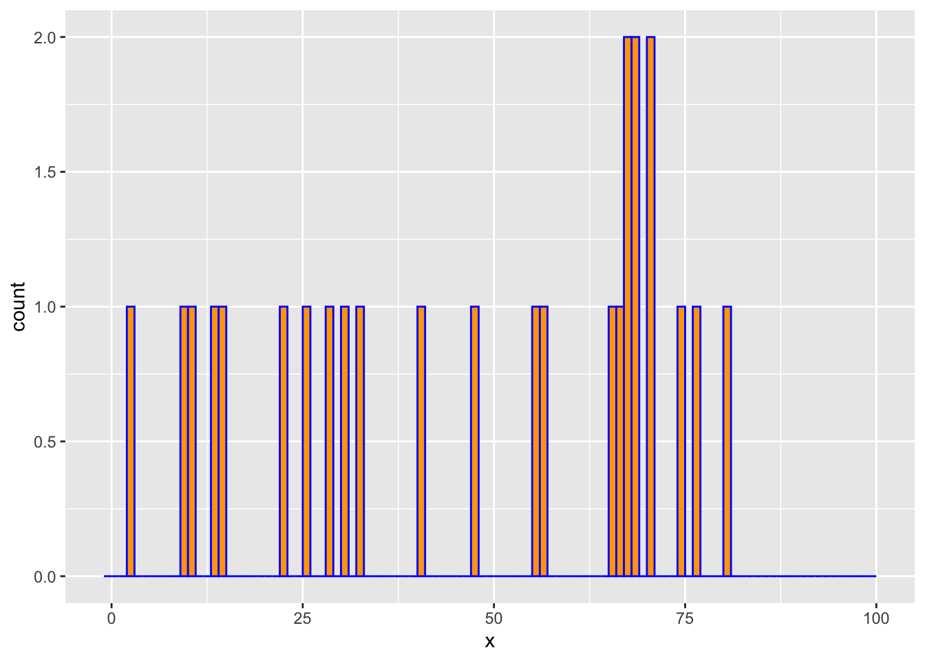
We now solve problem with log-concave constraint.
u <- Variable(K+1)
obj <- t(counts) %*% u
constraints <- list(sum(exp(u)) <= 1, diff(u[1:K]) >= diff(u[2:(K+1)]))
prob <- Problem(Maximize(obj), constraints)
result <- psolve(prob, solver = "SCS")
Warning: Solution may be inaccurate. Try another solver, adjusting the solver settings,
or solve with `verbose = TRUE` for more information.check_solver_status(prob)
pmf <- value(exp(u))The above lines transform the variables \(u_k\) to \(e^{u_k}\) before calculating their resulting values. This is possible because exp is a member of the CVXR library of atoms, so it can operate directly on a Variable object such as u.
Below are the comparison plots of pmf and cdf.
dens <- density(x, bw = "sj")
d <- data.frame(x = xrange, True = xprobs, Optimal = pmf,
                Empirical = approx(x = dens$x, y = dens$y, xout = xrange)$y)
plot.data <- gather(data = d, key = "Type", value = "Estimate", True, Empirical, Optimal,
                    factor_key = TRUE)
ggplot(plot.data) +
    geom_line(mapping = aes(x = x, y = Estimate, color = Type)) +
    theme(legend.position = "top")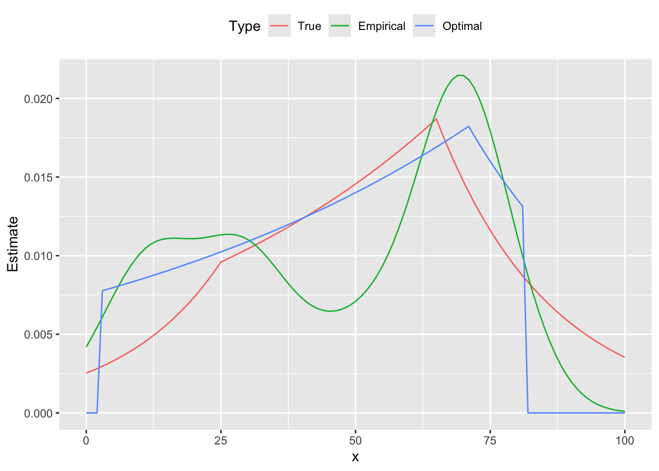
d <- data.frame(x = xrange, True = cumsum(xprobs),
                Empirical = cumsum(counts) / sum(counts),
                Optimal = cumsum(pmf))
plot.data <- gather(data = d, key = "Type", value = "Estimate", True, Empirical, Optimal,
                    factor_key = TRUE)
ggplot(plot.data) +
    geom_line(mapping = aes(x = x, y = Estimate, color = Type)) +
    theme(legend.position = "top")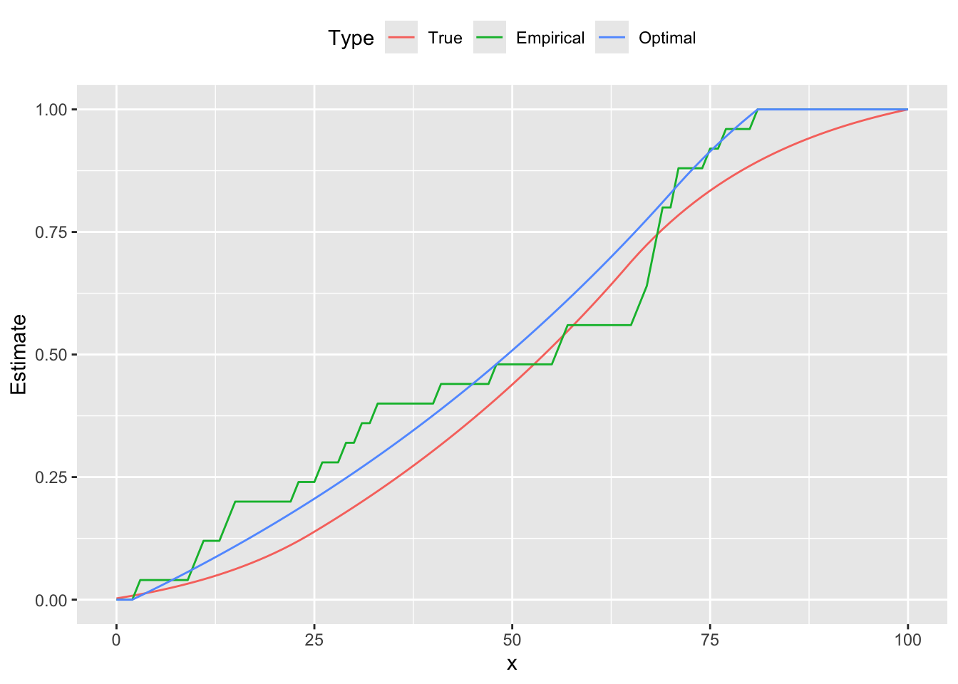
From the figures we see that the estimated curve is much closer to the true distribution, exhibiting a similar shape and number of peaks. In contrast, the empirical probability mass function oscillates, failing to be log-concave on parts of its domain. These differences are reflected in the cumulative distribution functions as well.
Session Info
R version 4.6.0 (2026-04-24)
Platform: aarch64-apple-darwin23
Running under: macOS Tahoe 26.5.1

Matrix products: default
BLAS:   /Library/Frameworks/R.framework/Versions/4.6/Resources/lib/libRblas.0.dylib
LAPACK: /Library/Frameworks/R.framework/Versions/4.6/Resources/lib/libRlapack.dylib;  LAPACK version 3.12.1

locale:
[1] en_US.UTF-8/en_US.UTF-8/en_US.UTF-8/C/en_US.UTF-8/en_US.UTF-8

time zone: America/Los_Angeles
tzcode source: internal

attached base packages:
[1] stats     graphics  grDevices utils     datasets  methods   base

other attached packages:
[1] tidyr_1.3.2   ggplot2_4.0.3 CVXR_1.9.1

loaded via a namespace (and not attached):
 [1] Matrix_1.7-5       gtable_0.3.6       jsonlite_2.0.0     dplyr_1.2.1
 [5] compiler_4.6.0     highs_1.14.0-2     tidyselect_1.2.1   Rcpp_1.1.1-1.1
 [9] dichromat_2.0-0.1  scales_1.4.0       yaml_2.3.12        fastmap_1.2.0
[13] clarabel_0.11.2    here_1.0.2         lattice_0.22-9     R6_2.6.1
[17] labeling_0.4.3     generics_0.1.4     knitr_1.51         htmlwidgets_1.6.4
[21] backports_1.5.1    checkmate_2.3.4    tibble_3.3.1       rprojroot_2.1.1
[25] osqp_1.0.0         pillar_1.11.1      RColorBrewer_1.1-3 rlang_1.2.0
[29] xfun_0.58          S7_0.2.2           otel_0.2.0         cli_3.6.6
[33] withr_3.0.2        magrittr_2.0.5     digest_0.6.39      grid_4.6.0
[37] gmp_0.7-5.1        lifecycle_1.0.5    scs_3.2.7          vctrs_0.7.3
[41] evaluate_1.0.5     glue_1.8.1         farver_2.1.2       purrr_1.2.2
[45] rmarkdown_2.31     pkgconfig_2.0.3    tools_4.6.0        htmltools_0.5.9