## Fix random number generator so we can repeat the experiment
set.seed(1)

## The threshold value below which we consider an element to be zero
delta <- 1e-8

## Problem dimensions (m inequalities in n-dimensional space)
m <- 100
n <- 50

## Construct a feasible set of inequalities
## (This system is feasible for the x0 point.)
A <- matrix(rnorm(m * n), nrow = m, ncol = n)
x0 <- rnorm(n)
b <- as.vector(A %*% x0) + runif(m)Sparse Solution of Linear Inequalities
Introduction
This example is adapted from the CVX example of the same name, by Almir Mutapcic (2/28/2006) and the CVXPY adaptation by Judson Wilson (5/11/2014).
Topic references:
- Section 6.2, Boyd & Vandenberghe, Convex Optimization.
- Tropp, J. A. “Just relax: Convex programming methods for subset selection and sparse approximation.”
We consider a set of linear inequalities \(Ax \preceq b\) which are feasible. We apply two heuristics to find a sparse point \(x\) that satisfies these inequalities.
The \(\ell_1\)-norm Heuristic
The standard \(\ell_1\)-norm heuristic for finding a sparse solution is:
\[ \begin{array}{ll} \mbox{minimize} & \|x\|_1 \\ \mbox{subject to} & Ax \preceq b. \end{array} \]
The Iterative Log Heuristic
The log-based heuristic is an iterative method for finding a sparse solution, by finding a local optimal point for the problem:
\[ \begin{array}{ll} \mbox{minimize} & \sum_i \log(\delta + |x_i|) \\ \mbox{subject to} & Ax \preceq b, \end{array} \]
where \(\delta\) is a small threshold value. Since this is a minimization of a concave function, it is not convex. However, we can apply a heuristic in which we linearize the objective, solve, and re-iterate. This becomes a weighted \(\ell_1\)-norm heuristic:
\[ \begin{array}{ll} \mbox{minimize} & \sum_i W_i |x_i| \\ \mbox{subject to} & Ax \preceq b, \end{array} \]
which in each iteration re-adjusts the weights \(W_i\) based on the rule \(W_i = 1 / (\delta + |x_i|)\).
This algorithm is described in:
- Rao, B. D. and Kreutz-Delgado, K. “An affine scaling methodology for best basis selection.”
- Lobo, M. S., Fazel, M. and Boyd, S. “Portfolio optimization with linear and fixed transaction costs.”
Generate Problem Data
\(\ell_1\)-norm Heuristic
## Create variable
x_l1 <- Variable(n)

## Create constraint
constraints <- list(A %*% x_l1 <= b)

## Form objective
obj <- Minimize(p_norm(x_l1, 1))

## Form and solve problem
prob <- Problem(obj, constraints)
result_l1 <- psolve(prob)
cat(sprintf("Status: %s\n", status(prob)))

## Number of nonzero elements in the solution
x_l1_val <- as.numeric(value(x_l1))
nnz_l1 <- sum(abs(x_l1_val) > delta)
cat(sprintf("Found a feasible x in R^%d that has %d nonzeros.\n", n, nnz_l1))
cat(sprintf("Optimal objective value: %.6f\n", result_l1))
Status: optimal
Found a feasible x in R^50 that has 44 nonzeros.
Optimal objective value: 33.986486Iterative Log Heuristic
## Do 15 iterations
NUM_RUNS <- 15
nnzs_log <- numeric(NUM_RUNS)

## Store W as a numeric vector for weights
W <- rep(1, n)
x_log <- Variable(n)

for (k in seq_len(NUM_RUNS)) {
    ## Form and solve the weighted l1 problem
    obj <- Minimize(t(W) %*% abs(x_log))
    constraints <- list(A %*% x_log <= b)
    prob <- Problem(obj, constraints)

    ## Solve
    result_log <- psolve(prob)

    prob_status <- status(prob)
    if (!prob_status %in% c("optimal", "optimal_inaccurate")) {
        stop(sprintf("Solver did not converge (status: %s)", prob_status))
    }

    ## Get current solution
    x_log_val <- as.numeric(value(x_log))

    ## Display new number of nonzeros in the solution vector
    nnz <- sum(abs(x_log_val) > delta)
    nnzs_log[k] <- nnz
    cat(sprintf("Iteration %d: Found a feasible x in R^%d with %d nonzeros...\n",
                k, n, nnz))

    ## Adjust the weights elementwise and re-iterate
    W <- 1 / (delta + abs(x_log_val))
}
Iteration 1: Found a feasible x in R^50 with 44 nonzeros...
Iteration 2: Found a feasible x in R^50 with 41 nonzeros...
Iteration 3: Found a feasible x in R^50 with 38 nonzeros...
Iteration 4: Found a feasible x in R^50 with 38 nonzeros...
Iteration 5: Found a feasible x in R^50 with 38 nonzeros...
Iteration 6: Found a feasible x in R^50 with 38 nonzeros...
Iteration 7: Found a feasible x in R^50 with 38 nonzeros...
Iteration 8: Found a feasible x in R^50 with 38 nonzeros...
Iteration 9: Found a feasible x in R^50 with 38 nonzeros...
Iteration 10: Found a feasible x in R^50 with 37 nonzeros...
Iteration 11: Found a feasible x in R^50 with 37 nonzeros...
Iteration 12: Found a feasible x in R^50 with 36 nonzeros...
Iteration 13: Found a feasible x in R^50 with 36 nonzeros...
Iteration 14: Found a feasible x in R^50 with 36 nonzeros...
Iteration 15: Found a feasible x in R^50 with 36 nonzeros...Result Plot
The following plot shows the result of the \(\ell_1\)-norm heuristic, as well as the result for each iteration of the log heuristic.
df_plot <- data.frame(
    iteration = 1:NUM_RUNS,
    log_heuristic = nnzs_log
)

ggplot(df_plot, aes(x = iteration, y = log_heuristic)) +
    geom_line(aes(color = "Log heuristic")) +
    geom_point(aes(color = "Log heuristic")) +
    geom_hline(aes(yintercept = nnz_l1, color = "l1-norm heuristic"),
               linetype = "dashed") +
    coord_cartesian(xlim = c(1, NUM_RUNS), ylim = c(0, n)) +
    labs(x = "Iteration", y = "Number of non-zeros (cardinality)",
         color = "") +
    theme_minimal() +
    theme(legend.position = "bottom")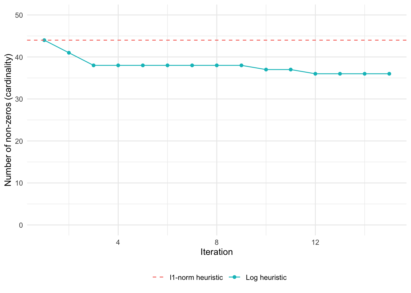
The iterative log heuristic converges to a sparser solution than the \(\ell_1\)-norm heuristic.
Session Info
R version 4.6.0 (2026-04-24)
Platform: aarch64-apple-darwin23
Running under: macOS Tahoe 26.5.1

Matrix products: default
BLAS:   /Library/Frameworks/R.framework/Versions/4.6/Resources/lib/libRblas.0.dylib
LAPACK: /Library/Frameworks/R.framework/Versions/4.6/Resources/lib/libRlapack.dylib;  LAPACK version 3.12.1

locale:
[1] en_US.UTF-8/en_US.UTF-8/en_US.UTF-8/C/en_US.UTF-8/en_US.UTF-8

time zone: America/Los_Angeles
tzcode source: internal

attached base packages:
[1] stats     graphics  grDevices utils     datasets  methods   base

other attached packages:
[1] ggplot2_4.0.3 CVXR_1.9.1

loaded via a namespace (and not attached):
 [1] piqp_0.6.2         Matrix_1.7-5       gtable_0.3.6       jsonlite_2.0.0
 [5] dplyr_1.2.1        compiler_4.6.0     highs_1.14.0-2     tidyselect_1.2.1
 [9] Rcpp_1.1.1-1.1     slam_0.1-55        cccp_0.3-3         dichromat_2.0-0.1
[13] scales_1.4.0       yaml_2.3.12        fastmap_1.2.0      clarabel_0.11.2
[17] lattice_0.22-9     R6_2.6.1           labeling_0.4.3     generics_0.1.4
[21] knitr_1.51         htmlwidgets_1.6.4  backports_1.5.1    checkmate_2.3.4
[25] tibble_3.3.1       osqp_1.0.0         pillar_1.11.1      RColorBrewer_1.1-3
[29] rlang_1.2.0        xfun_0.58          S7_0.2.2           otel_0.2.0
[33] cli_3.6.6          withr_3.0.2        magrittr_2.0.5     Rglpk_0.6-5.1
[37] digest_0.6.39      grid_4.6.0         gmp_0.7-5.1        lifecycle_1.0.5
[41] ECOSolveR_0.6.1    scs_3.2.7          vctrs_0.7.3        evaluate_1.0.5
[45] glue_1.8.1         farver_2.1.2       codetools_0.2-20   rmarkdown_2.31
[49] pkgconfig_2.0.3    tools_4.6.0        htmltools_0.5.9
References
- Boyd, S. and Vandenberghe, L. (2004). Convex Optimization. Cambridge University Press. Section 6.2.
- Tropp, J. A. (2006). “Just relax: Convex programming methods for subset selection and sparse approximation.” IEEE Transactions on Information Theory, 52(3), 1030–1051.
- Rao, B. D. and Kreutz-Delgado, K. (1999). “An affine scaling methodology for best basis selection.” IEEE Transactions on Signal Processing, 47(1), 187–200.