Sparse Inverse Covariance Estimation

Author

Anqi Fu and Balasubramanian Narasimhan

Introduction

Assume we are given i.i.d. observations \(x_i \sim N(0,\Sigma)\) for \(i = 1,\ldots,m\), and the covariance matrix \(\Sigma \in {\mathbf S}_+^n\), the set of symmetric positive semidefinite matrices, has a sparse inverse \(S = \Sigma^{-1}\). Let \(Q = \frac{1}{m-1}\sum_{i=1}^m (x_i - \bar x)(x_i - \bar x)^T\) be our sample covariance. One way to estimate \(\Sigma\) is to maximize the log-likelihood with the prior knowledge that \(S\) is sparse (Friedman et al. 2008), which amounts to the optimization problem:

\[ \begin{array}{ll} \underset{S}{\mbox{maximize}} & \log\det(S) - \mbox{tr}(SQ) \\ \mbox{subject to} & S \in {\mathbf S}_+^n, \quad \sum_{i=1}^n \sum_{j=1}^n |S_{ij}| \leq \alpha. \end{array} \]

The parameter \(\alpha \geq 0\) controls the degree of sparsity. The problem is convex, so we can solve it using CVXR.

Example

We’ll create a sparse positive semi-definite matrix \(S\) using synthetic data

set.seed(1)
n <- 10      ## Dimension of matrix
m <- 1000    ## Number of samples

## Create sparse, symmetric PSD matrix S
A <- rsparsematrix(n, n, 0.15, rand.x = stats::rnorm)
Strue <- A %*% t(A) + 0.05 * diag(rep(1, n))    ## Force matrix to be strictly positive definite

We can now create the covariance matrix \(R\) as the inverse of \(S\).

R <- base::solve(Strue)

As test data, we sample from a multivariate normal with the fact that if \(Y \sim N(0, I)\), then \(R^{1/2}Y \sim N(0, R)\) since \(R\) is symmetric.

x_sample <- matrix(stats::rnorm(n * m), nrow = m, ncol = n) %*% t(expm::sqrtm(R))
Q <- cov(x_sample)    ## Sample covariance matrix

Finally, we solve our convex program for a set of \(\alpha\) values.

Positive semi-definite variables are designated using PSD = TRUE.

alphas <- c(10, 8, 6, 4, 1)
S <- Variable(c(n, n), PSD = TRUE)

obj <- Maximize(log_det(S) - matrix_trace(S %*% Q))

S.est <- lapply(alphas,
                function(alpha) {
                    constraints <- list(sum(abs(S)) <= alpha)
                    ## Form and solve optimization problem
                    prob <- Problem(obj, constraints)
                    result <- psolve(prob)
                    check_solver_status(prob)

                    ## Create covariance matrix
                    R_hat <- base::solve(value(S))
                    Sres <- value(S)
                    Sres[abs(Sres) <= 1e-4] <- 0
                    Sres
                })

In the code above, the PSD = TRUE attribute restricts S to the positive semidefinite cone. In our objective, we use CVXR functions for the log-determinant and trace. The expression matrix_trace(S %*% Q) is equivalent to `sum(diag(S %*% Q))}, but the former is preferred because it is more efficient than making nested function calls.

However, a standalone atom does not exist for the determinant, so we cannot replace log_det(S) with log(det(S)) since det is undefined for a PSD variable object.

Results

The figures below depict the solutions for the above dataset with \(m = 1000, n = 10\), and \(S\) containing 26% non-zero entries, represented by the dark squares in the images below. The sparsity of our inverse covariance estimate decreases for higher \(\alpha\), so that when \(\alpha = 1\), most of the off-diagonal entries are zero, while if \(\alpha = 10\), over half the matrix is dense. At \(\alpha = 4\), we achieve the true percentage of non-zeros.

do.call(multiplot, args = c(list(plotSpMat(Strue)),
                            mapply(plotSpMat, S.est, alphas, SIMPLIFY = FALSE),
                            list(layout = matrix(1:6, nrow = 2, byrow = TRUE))))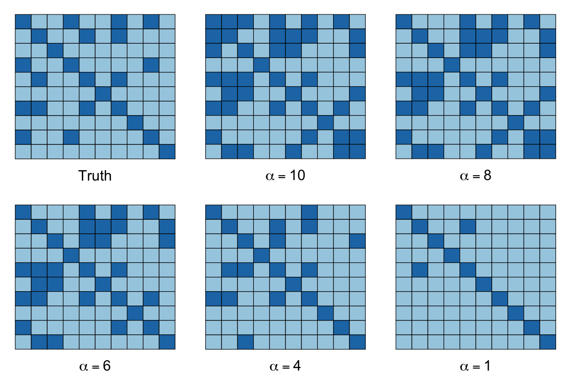

Session Info

R version 4.6.0 (2026-04-24)
Platform: aarch64-apple-darwin23
Running under: macOS Tahoe 26.5.1

Matrix products: default
BLAS:   /Library/Frameworks/R.framework/Versions/4.6/Resources/lib/libRblas.0.dylib 
LAPACK: /Library/Frameworks/R.framework/Versions/4.6/Resources/lib/libRlapack.dylib;  LAPACK version 3.12.1

locale:
[1] en_US.UTF-8/en_US.UTF-8/en_US.UTF-8/C/en_US.UTF-8/en_US.UTF-8

time zone: America/Los_Angeles
tzcode source: internal

attached base packages:
[1] grid      stats     graphics  grDevices utils     datasets  methods  
[8] base     

other attached packages:
[1] expm_1.0-0    Matrix_1.7-5  ggplot2_4.0.3 CVXR_1.9.1   

loaded via a namespace (and not attached):
 [1] piqp_0.6.2         gtable_0.3.6       jsonlite_2.0.0     dplyr_1.2.1       
 [5] compiler_4.6.0     highs_1.12.0-3     tidyselect_1.2.1   Rcpp_1.1.1-1.1    
 [9] slam_0.1-55        cccp_0.3-3         dichromat_2.0-0.1  scales_1.4.0      
[13] yaml_2.3.12        fastmap_1.2.0      clarabel_0.11.2    here_1.0.2        
[17] lattice_0.22-9     R6_2.6.1           labeling_0.4.3     generics_0.1.4    
[21] knitr_1.51         htmlwidgets_1.6.4  backports_1.5.1    checkmate_2.3.4   
[25] tibble_3.3.1       rprojroot_2.1.1    osqp_1.0.0         pillar_1.11.1     
[29] RColorBrewer_1.1-3 rlang_1.2.0        xfun_0.57          S7_0.2.2          
[33] otel_0.2.0         cli_3.6.6          withr_3.0.2        magrittr_2.0.5    
[37] Rglpk_0.6-5.1      digest_0.6.39      gmp_0.7-5.1        lifecycle_1.0.5   
[41] ECOSolveR_0.6.1    scs_3.2.7          vctrs_0.7.3        evaluate_1.0.5    
[45] glue_1.8.1         farver_2.1.2       codetools_0.2-20   rmarkdown_2.31    
[49] pkgconfig_2.0.3    tools_4.6.0        htmltools_0.5.9

References

Friedman, J., T. Hastie, and R. Tibshirani. 2008. “Sparse Inverse Covariance Estimation with the Graphical Lasso.” Biostatistics 9 (3): 432–41.