Aerospace Design via Quasiconvex Optimization

Author

CVXPY Developers and Balasubramanian Narasimhan

Introduction

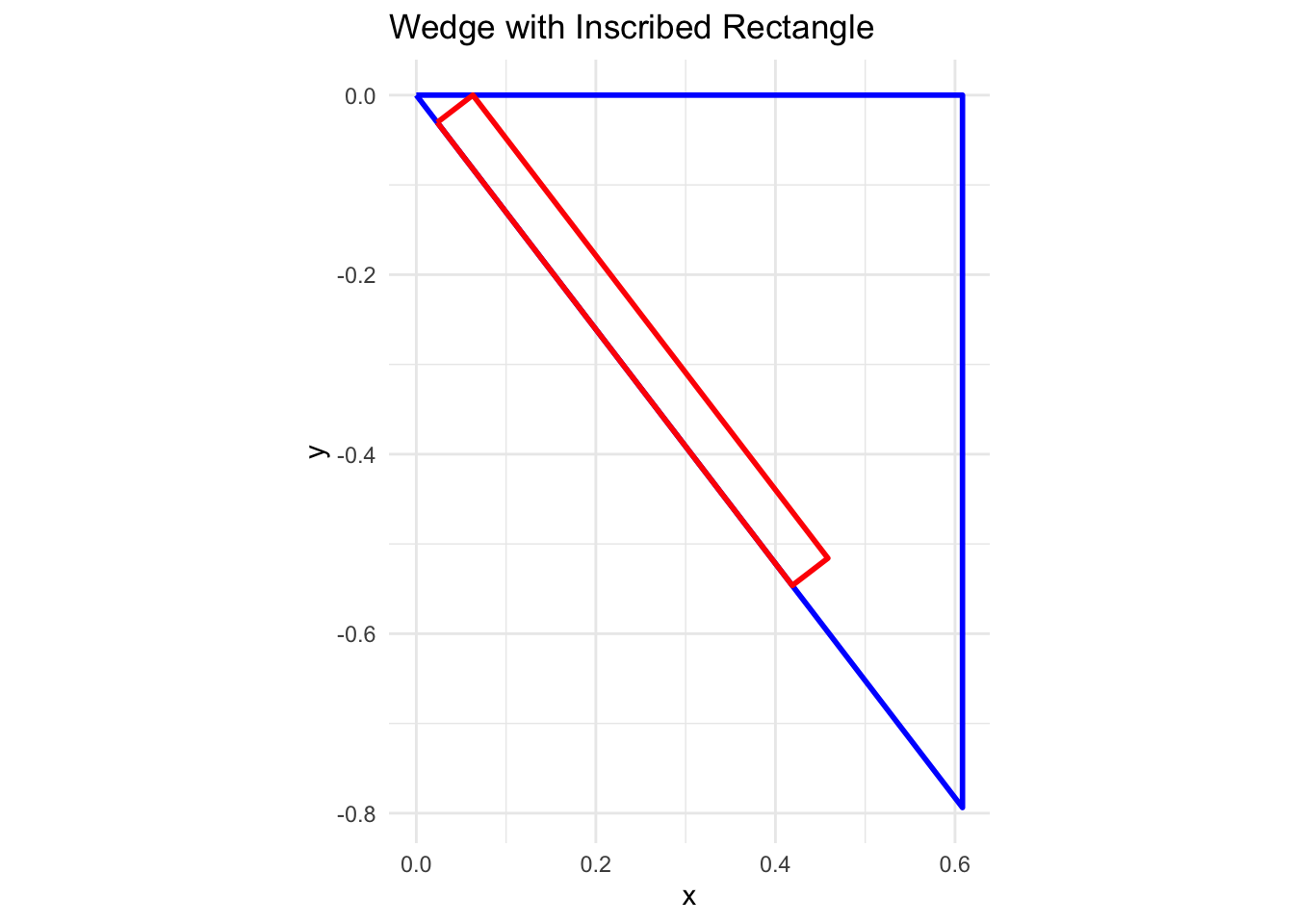
Consider a triangle, or a wedge, located within a hypersonic flow. A standard aerospace design optimization problem is to design the wedge to maximize the lift-to-drag ratio (L/D) (or conversely minimize the D/L ratio), subject to certain geometric constraints. In this example, the wedge is known to have a constant hypotenuse, and our job is to choose its width and height.

Problem Formulation

The drag-to-lift ratio is given by

\[ \frac{D}{L} = \frac{c_d}{c_l}, \]

where \(c_d\) and \(c_l\) are drag and lift coefficients, respectively, that are obtained by integrating the projection of the pressure coefficient in directions parallel to, and perpendicular to, the body.

We will assume the pressure coefficient is given by the Newtonian sine-squared law for whetted areas of the body,

\[ c_p = 2(\hat{v} \cdot \hat{n})^2 \]

and elsewhere \(c_p = 0\). Here, \(\hat{v}\) is the free stream direction, which for simplicity we assume is parallel to the body so that \(\hat{v} = \langle 1, 0 \rangle\), and \(\hat{n}\) is the local unit normal. For a wedge defined by width \(\Delta x\) and height \(\Delta y\),

\[ \hat{n} = \langle -\Delta y / s, -\Delta x / s \rangle \]

where \(s\) is the hypotenuse length. Therefore,

\[ c_p = 2\left(\frac{-\Delta y}{s}\right)^2 = \frac{2 \Delta y^2}{s^2}. \]

The lift and drag coefficients are given by

\[ \begin{aligned} c_d &= \frac{1}{c}\int_0^s -c_p \hat{n}_x \, ds \\ c_l &= \frac{1}{c}\int_0^s -c_p \hat{n}_y \, ds \end{aligned} \]

where \(c\) is the reference chord length of the body. Given that \(\hat{n}\) and therefore \(c_p\) are constant over the whetted surface of the body,

\[ \begin{aligned} c_d &= \frac{s}{c} \frac{2 \Delta y^2}{s^2} \frac{\Delta y}{s} \\ c_l &= \frac{s}{c} \frac{2 \Delta y^2}{s^2} \frac{\Delta x}{s} \end{aligned} \]

Assuming \(s = 1\), so that \(\Delta y = \sqrt{1 - \Delta x^2}\), plugging in the above into the equation for \(D/L\), we obtain

\[ \frac{D}{L} = \frac{\Delta y}{\Delta x} = \frac{\sqrt{1 - \Delta x^2}}{\Delta x} = \sqrt{\frac{1}{\Delta x^2} - 1}. \]

This function is representable as a DQCP quasilinear function.

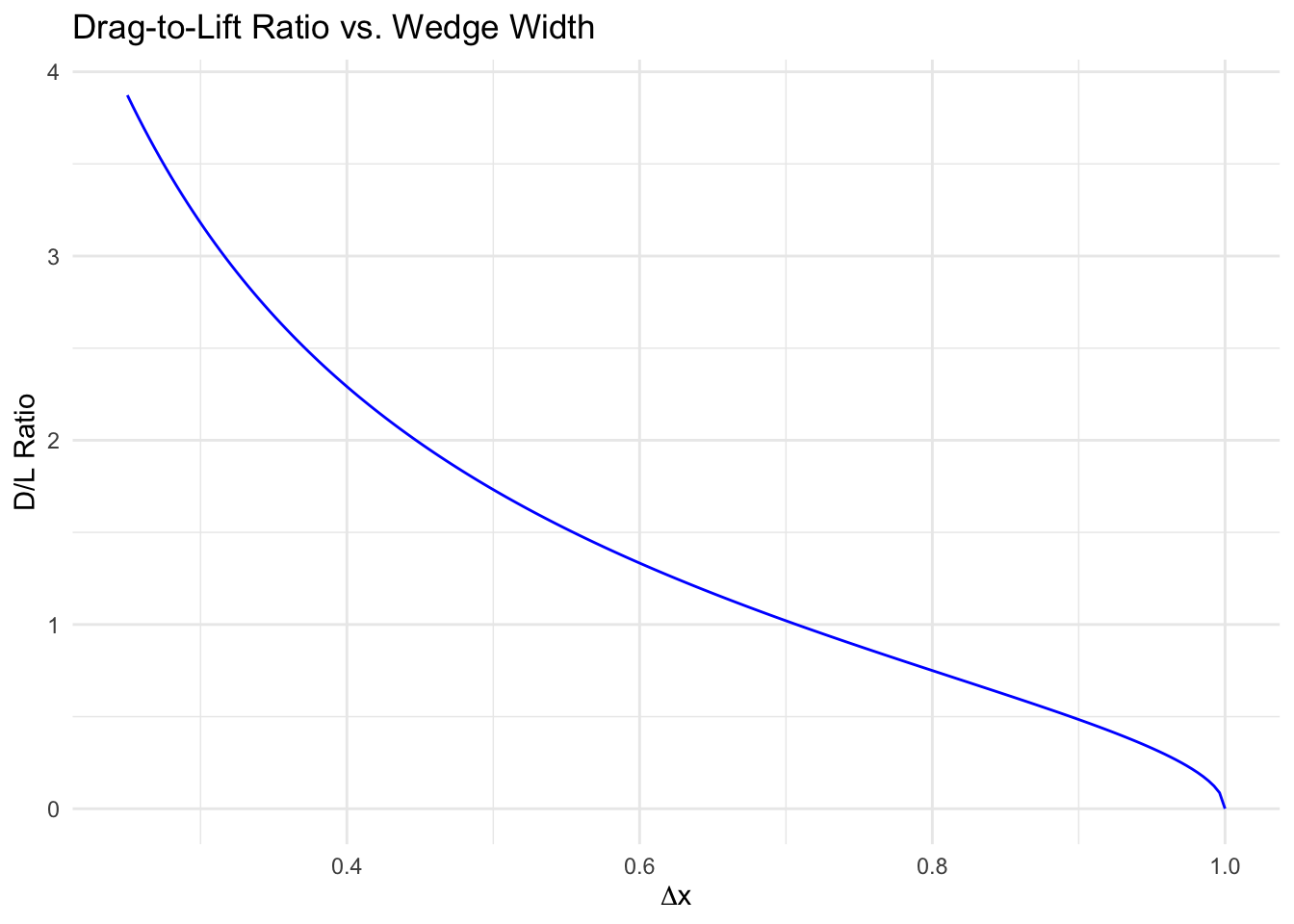
Plotting the Objective

We can visualize the D/L ratio as a function of \(\Delta x\):

x_vals <- seq(0.25, 1, length.out = 201)
obj_vals <- sqrt(1 / x_vals^2 - 1)
ggplot(data.frame(x = x_vals, y = obj_vals), aes(x, y)) +
    geom_line(color = "blue") +
    labs(x = expression(Delta * x), y = "D/L Ratio",
         title = "Drag-to-Lift Ratio vs. Wedge Width") +
    theme_minimal()

DQCP Formulation

We now express the objective in CVXR and verify its curvature:

x <- Variable(pos = TRUE)
obj <- sqrt(inv_pos(power(x, 2)) - 1)
cat("This objective function is", curvature(obj), "\n")
This objective function is UNKNOWN 

Minimizing this objective function subject to constraints representing payload requirements is a standard aerospace design problem. In this case we consider the constraint that the wedge must be able to contain a rectangle of given length and width internally along its hypotenuse. This is representable as a convex constraint.

a <- 0.05  # height of rectangle (should be at most b)
b <- 0.65  # width of rectangle
constraint <- list(a * inv_pos(x) - (1 - b) * sqrt(1 - power(x, 2)) <= 0)

Solving the Problem

prob <- Problem(Minimize(obj), constraint)
result <- psolve(prob, qcp = TRUE)
check_solver_status(prob)
ld_ratio <- 1 / result
x_opt <- value(x)
y_opt <- sqrt(1 - x_opt^2)
cat("Final L/D Ratio:", ld_ratio, "\n")
cat("Final width of wedge:", x_opt, "\n")
cat("Final height of wedge:", y_opt, "\n")
Final L/D Ratio: 0.7664405 
Final width of wedge: 0.6083185 
Final height of wedge: 0.793693 

Verification Plot

Once the solution has been found, we can create a plot to verify that the rectangle is inscribed within the wedge.

y <- sqrt(1 - x_opt^2)
lambda1 <- a * x_opt / y

## Wedge vertices
wedge <- data.frame(
    x = c(0, x_opt, x_opt, 0),
    y = c(0, 0, -y, 0)
)

## Rectangle vertices
pt1 <- c(lambda1 * x_opt, -lambda1 * y)
pt2 <- c((lambda1 + b) * x_opt, -(lambda1 + b) * y)
pt3 <- c((lambda1 + b) * x_opt + a * y, -(lambda1 + b) * y + a * x_opt)
pt4 <- c(lambda1 * x_opt + a * y, -lambda1 * y + a * x_opt)
rect <- data.frame(
    x = c(pt1[1], pt2[1], pt3[1], pt4[1], pt1[1]),
    y = c(pt1[2], pt2[2], pt3[2], pt4[2], pt1[2])
)

ggplot() +
    geom_path(data = wedge, aes(x, y), color = "blue", linewidth = 1) +
    geom_path(data = rect, aes(x, y), color = "red", linewidth = 1) +
    coord_fixed() +
    labs(title = "Wedge with Inscribed Rectangle") +
    theme_minimal()

Session Info

R version 4.5.3 (2026-03-11)
Platform: aarch64-apple-darwin20
Running under: macOS Tahoe 26.3.1

Matrix products: default
BLAS:   /Library/Frameworks/R.framework/Versions/4.5-arm64/Resources/lib/libRblas.0.dylib 
LAPACK: /Library/Frameworks/R.framework/Versions/4.5-arm64/Resources/lib/libRlapack.dylib;  LAPACK version 3.12.1

locale:
[1] en_US.UTF-8/en_US.UTF-8/en_US.UTF-8/C/en_US.UTF-8/en_US.UTF-8

time zone: America/Los_Angeles
tzcode source: internal

attached base packages:
[1] stats     graphics  grDevices utils     datasets  methods   base     

other attached packages:
[1] ggplot2_4.0.2 CVXR_1.8.1   

loaded via a namespace (and not attached):
 [1] gmp_0.7-5.1        generics_0.1.4     clarabel_0.11.2    slam_0.1-55       
 [5] lattice_0.22-9     digest_0.6.39      magrittr_2.0.4     evaluate_1.0.5    
 [9] grid_4.5.3         RColorBrewer_1.1-3 fastmap_1.2.0      rprojroot_2.1.1   
[13] jsonlite_2.0.0     Matrix_1.7-4       ECOSolveR_0.6.1    backports_1.5.0   
[17] scs_3.2.7          Rmosek_11.1.1      scales_1.4.0       codetools_0.2-20  
[21] cli_3.6.5          rlang_1.1.7        Rglpk_0.6-5.1      withr_3.0.2       
[25] yaml_2.3.12        otel_0.2.0         tools_4.5.3        osqp_1.0.0        
[29] checkmate_2.3.4    dplyr_1.2.0        here_1.0.2         gurobi_13.0-1     
[33] vctrs_0.7.1        R6_2.6.1           lifecycle_1.0.5    htmlwidgets_1.6.4 
[37] pkgconfig_2.0.3    cccp_0.3-3         pillar_1.11.1      gtable_0.3.6      
[41] glue_1.8.0         Rcpp_1.1.1         xfun_0.56          tibble_3.3.1      
[45] tidyselect_1.2.1   knitr_1.51         dichromat_2.0-0.1  highs_1.12.0-3    
[49] farver_2.1.2       htmltools_0.5.9    labeling_0.4.3     rmarkdown_2.30    
[53] piqp_0.6.2         compiler_4.5.3     S7_0.2.1          

References

  • Agrawal, A., Boyd, S. (2020). Disciplined Quasiconvex Programming. Optimization Letters, 14, 1643–1657.