Direct Standardization

Author

Anqi Fu and Balasubramanian Narasimhan

Introduction

Consider a set of observations $(x_{i}, y_{i})$ drawn non-uniformly from an unknown distribution. We know the expected value of the columns of $X$ , denoted by $b \in R^{n}$ , and want to estimate the true distribution of $y$ . This situation may arise, for instance, if we wish to analyze the health of a population based on a sample skewed toward young males, knowing the average population-level sex, age, etc. The empirical distribution that places equal probability $1 / m$ on each $y_{i}$ is not a good estimate.

So, we must determine the weights $w \in R^{m}$ of a weighted empirical distribution, $y = y_{i}$ with probability $w_{i}$ , which rectifies the skewness of the sample (Fleiss, Levin, and Paik 2003, 19.5). We can pose this problem as

$\begin{array}{ll} \underset{w}{maximize} & \sum_{i = 1}^{m} - w_{i} \log w_{i} \\ subject to & w \geq 0, \sum_{i = 1}^{m} w_{i} = 1, X^{T} w = b . \end{array}$

Our objective is the total entropy, which is concave on $R_{+}^{m}$ , and our constraints ensure $w$ is a probability distribution that implies our known expectations on $X$ .

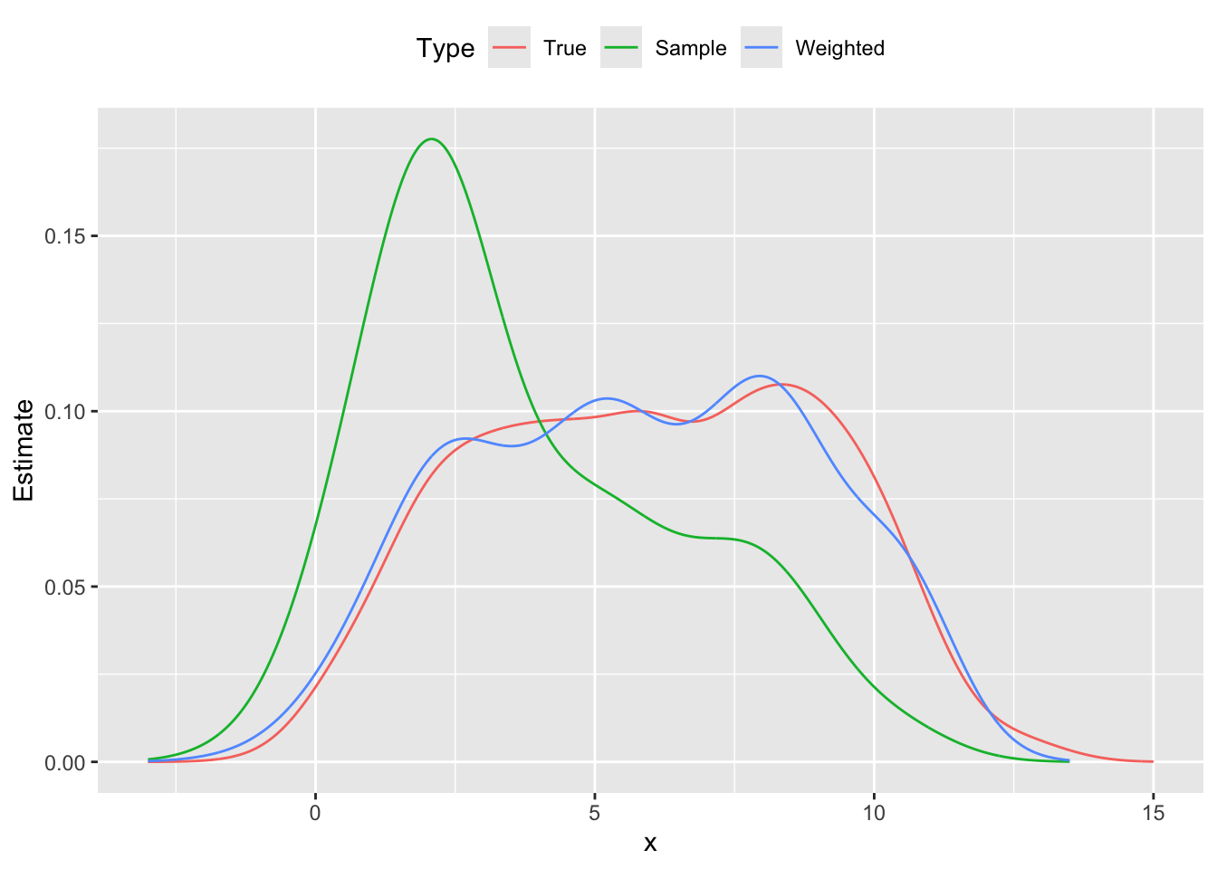
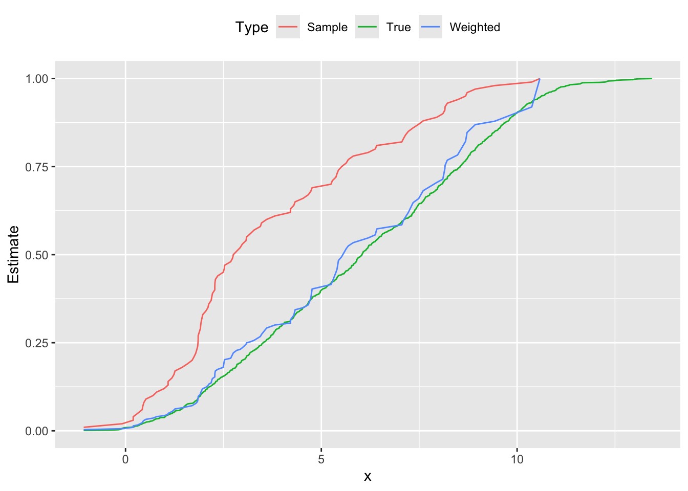
To illustrate this method, we generate $m = 1000$ data points $x_{i, 1} \sim Bernoulli (0.5)$ , $x_{i, 2} \sim Uniform (10, 60)$ , and $y_{i} \sim N (5 x_{i, 1} + 0.1 x_{i, 2}, 1)$ . Then we construct a skewed sample of $m = 100$ points that overrepresent small values of $y_{i}$ , thus biasing its distribution downwards. This can be seen in Figure $???$ , where the sample probability distribution peaks around $y = 2.0$ , and its cumulative distribution is shifted left from the population’s curve. Using direct standardization, we estimate $w_{i}$ and reweight our sample; the new empirical distribution cleaves much closer to the true distribution shown in red.

In the CVXR code below, we import data from the package and solve for $w$ .

## Import problem data
data(dspop)   # Population
data(dssamp)  # Skewed sample

ypop <- dspop[,1]
Xpop <- dspop[,-1]
y <- dssamp[,1]
X <- dssamp[,-1]
m <- nrow(X)

## Given population mean of features
b <- as.matrix(apply(Xpop, 2, mean))

## Construct the direct standardization problem
w <- Variable(m)
objective <- sum(entr(w))
constraints <- list(w >= 0, sum(w) == 1, t(X) %*% w == b)
prob <- Problem(Maximize(objective), constraints)

## Solve for the distribution weights
## psolve() returns the optimal value directly; variable values via value()
## (The deprecated solve() pattern result$getValue(x) still works but warns.)
result <- psolve(prob)
check_solver_status(prob)
weights <- value(w)
cat(sprintf("Optimal value: %f\n", result))

Optimal value: 4.223305

We can plot the density functions using linear approximations for the range of $y$ .

## Plot probability density functions
dens1 <- density(ypop)
dens2 <- density(y)
dens3 <- density(y, weights = weights)

Warning in density.default(y, weights = weights): Selecting bandwidth *not*
using 'weights'

yrange <- seq(-3, 15, 0.01)
d <- data.frame(x = yrange,
                True = approx(x = dens1$x, y = dens1$y, xout = yrange)$y,
                Sample = approx(x = dens2$x, y = dens2$y, xout = yrange)$y,
                Weighted = approx(x = dens3$x, y = dens3$y, xout = yrange)$y)
plot.data <- gather(data = d, key = "Type", value = "Estimate", True, Sample, Weighted,
                    factor_key = TRUE)
ggplot(plot.data) +
    geom_line(mapping = aes(x = x, y = Estimate, color = Type)) +
    theme(legend.position = "top")

Warning: Removed 300 rows containing missing values or values outside the scale range
(`geom_line()`).

Probability distribution functions population, skewed sample and reweighted sample

Followed by the cumulative distribution function.

## Return the cumulative distribution function
get_cdf <- function(data, probs, color = 'k') {
    if(missing(probs))
        probs <- rep(1.0/length(data), length(data))
    distro <- cbind(data, probs)
    dsort <- distro[order(distro[,1]),]
    ecdf <- base::cumsum(dsort[,2])
    cbind(dsort[,1], ecdf)
}

## Plot cumulative distribution functions
d1 <- data.frame("True", get_cdf(ypop))
d2 <- data.frame("Sample", get_cdf(y))
d3 <- data.frame("Weighted", get_cdf(y, weights))

names(d1) <- names(d2) <- names(d3) <- c("Type", "x", "Estimate")
plot.data <- rbind(d1, d2, d3)

ggplot(plot.data) +
    geom_line(mapping = aes(x = x, y = Estimate, color = Type)) +
    theme(legend.position = "top")

Session Info

R version 4.5.2 (2025-10-31)
Platform: aarch64-apple-darwin20
Running under: macOS Tahoe 26.3.1

Matrix products: default
BLAS:   /Library/Frameworks/R.framework/Versions/4.5-arm64/Resources/lib/libRblas.0.dylib 
LAPACK: /Library/Frameworks/R.framework/Versions/4.5-arm64/Resources/lib/libRlapack.dylib;  LAPACK version 3.12.1

locale:
[1] en_US.UTF-8/en_US.UTF-8/en_US.UTF-8/C/en_US.UTF-8/en_US.UTF-8

time zone: America/Los_Angeles
tzcode source: internal

attached base packages:
[1] stats     graphics  grDevices utils     datasets  methods   base     

other attached packages:
[1] tidyr_1.3.2   ggplot2_4.0.2 CVXR_1.8.1   

loaded via a namespace (and not attached):
 [1] gmp_0.7-5.1        generics_0.1.4     clarabel_0.11.2    slam_0.1-55       
 [5] lattice_0.22-9     digest_0.6.39      magrittr_2.0.4     evaluate_1.0.5    
 [9] grid_4.5.2         RColorBrewer_1.1-3 fastmap_1.2.0      rprojroot_2.1.1   
[13] jsonlite_2.0.0     Matrix_1.7-4       ECOSolveR_0.6.1    backports_1.5.0   
[17] scs_3.2.7          purrr_1.2.1        Rmosek_11.1.1      scales_1.4.0      
[21] codetools_0.2-20   cli_3.6.5          rlang_1.1.7        Rglpk_0.6-5.1     
[25] withr_3.0.2        yaml_2.3.12        otel_0.2.0         tools_4.5.2       
[29] osqp_1.0.0         Rcplex_0.3-8       checkmate_2.3.4    dplyr_1.2.0       
[33] here_1.0.2         gurobi_13.0-1      vctrs_0.7.1        R6_2.6.1          
[37] lifecycle_1.0.5    htmlwidgets_1.6.4  pkgconfig_2.0.3    cccp_0.3-3        
[41] pillar_1.11.1      gtable_0.3.6       glue_1.8.0         Rcpp_1.1.1        
[45] xfun_0.56          tibble_3.3.1       tidyselect_1.2.1   knitr_1.51        
[49] dichromat_2.0-0.1  highs_1.12.0-3     farver_2.1.2       htmltools_0.5.9   
[53] labeling_0.4.3     rmarkdown_2.30     piqp_0.6.2         compiler_4.5.2    
[57] S7_0.2.1

References

Fleiss, J. L., B. Levin, and M. C. Paik. 2003. Statistical Methods for Rates and Proportions. Wiley-Interscience.