Robust Kalman Filtering for Vehicle Tracking

Author

CVXPY Developers and Balasubramanian Narasimhan

Introduction

We will try to pinpoint the location of a moving vehicle with high accuracy from noisy sensor data. We do this by modeling the vehicle state as a discrete-time linear dynamical system. Standard Kalman filtering can be used to approach this problem when the sensor noise is assumed to be Gaussian. We use robust Kalman filtering to get a more accurate estimate of the vehicle state for a non-Gaussian case with outliers.

Problem Statement

A discrete-time linear dynamical system consists of a sequence of state vectors $x_{t} \in R^{n}$ , indexed by time $t \in {0, \dots, N - 1}$ and dynamics equations

$\begin{aligned} x_{t + 1} & = A x_{t} + B w_{t} \\ y_{t} & = C x_{t} + v_{t}, \end{aligned}$

where $w_{t} \in R^{m}$ is an input to the dynamical system (say, a drive force on the vehicle), $y_{t} \in R^{r}$ is a state measurement, $v_{t} \in R^{r}$ is noise, $A$ is the drift matrix, $B$ is the input matrix, and $C$ is the observation matrix.

Given $A$ , $B$ , $C$ , and $y_{t}$ for $t = 0, \dots, N - 1$ , the goal is to estimate $x_{t}$ for $t = 0, \dots, N - 1$ .

Kalman Filtering

A Kalman filter estimates $x_{t}$ by solving the optimization problem

$\begin{array}{ll} minimize & \sum_{t = 0}^{N - 1} (∥ w_{t} ∥_{2}^{2} + τ ∥ v_{t} ∥_{2}^{2}) \\ subject to & x_{t + 1} = A x_{t} + B w_{t}, t = 0, \dots, N - 1 \\ y_{t} = C x_{t} + v_{t}, t = 0, \dots, N - 1, \end{array}$

where $τ$ is a tuning parameter. This problem is actually a least squares problem, and can be solved via linear algebra, without the need for more general convex optimization.

This model performs well when $w_{t}$ and $v_{t}$ are Gaussian. However, the quadratic objective can be influenced by large outliers, which degrades the accuracy of the recovery. To improve estimation in the presence of outliers, we can use robust Kalman filtering.

Robust Kalman Filtering

To handle outliers in $v_{t}$ , robust Kalman filtering replaces the quadratic cost with a Huber cost, which results in the convex optimization problem

$\begin{array}{ll} minimize & \sum_{t = 0}^{N - 1} (∥ w_{t} ∥_{2}^{2} + τ ϕ_{ρ} (v_{t})) \\ subject to & x_{t + 1} = A x_{t} + B w_{t}, t = 0, \dots, N - 1 \\ y_{t} = C x_{t} + v_{t}, t = 0, \dots, N - 1, \end{array}$

where $ϕ_{ρ}$ is the Huber function

$ϕ_{ρ} (a) = {\begin{cases} ∥ a ∥_{2}^{2} & ∥ a ∥_{2} \leq ρ \\ 2 ρ ∥ a ∥_{2} - ρ^{2} & ∥ a ∥_{2} > ρ . \end{cases}$

The Huber penalty function penalizes estimation error linearly outside of a ball of radius $ρ$ , whereas in standard Kalman filtering, all errors are penalized quadratically. Thus, large errors are penalized less harshly, making this model more robust to outliers.

Vehicle Tracking Example

We apply standard and robust Kalman filtering to a vehicle tracking problem with state $x_{t} \in R^{4}$ , where $(x_{t, 1}, x_{t, 2})$ is the position of the vehicle in two dimensions, and $(x_{t, 3}, x_{t, 4})$ is the vehicle velocity. The vehicle has unknown drive force $w_{t}$ , and we observe noisy measurements of the vehicle’s position, $y_{t} \in R^{2}$ .

The matrices for the dynamics are

$A = [\begin{matrix} 1 & 0 & (1 - \frac{γ}{2} Δ t) Δ t & 0 \\ 0 & 1 & 0 & (1 - \frac{γ}{2} Δ t) Δ t \\ 0 & 0 & 1 - γ Δ t & 0 \\ 0 & 0 & 0 & 1 - γ Δ t \end{matrix}],$

$B = [\begin{matrix} \frac{1}{2} Δ t^{2} & 0 \\ 0 & \frac{1}{2} Δ t^{2} \\ Δ t & 0 \\ 0 & Δ t \end{matrix}], C = [\begin{matrix} 1 & 0 & 0 & 0 \\ 0 & 1 & 0 & 0 \end{matrix}],$

where $γ$ is a velocity damping parameter.

Problem Data

We generate the data for the vehicle tracking problem. We have $N = 1000$ , $w_{t}$ a standard Gaussian, and $v_{t}$ a standard Gaussian, except $20 %$ of the points will be outliers with $σ = 20$ .

N <- 1000  # number of timesteps
T_end <- 50  # time will vary from 0 to T_end
ts <- seq(0, T_end, length.out = N)
delt <- ts[2] - ts[1]
gamma_damp <- 0.05  # damping, 0 is no damping

A <- matrix(0, 4, 4)
B <- matrix(0, 4, 2)
C <- matrix(0, 2, 4)

A[1,1] <- 1
A[2,2] <- 1
A[1,3] <- (1 - gamma_damp * delt / 2) * delt
A[2,4] <- (1 - gamma_damp * delt / 2) * delt
A[3,3] <- 1 - gamma_damp * delt
A[4,4] <- 1 - gamma_damp * delt

B[1,1] <- delt^2 / 2
B[2,2] <- delt^2 / 2
B[3,1] <- delt
B[4,2] <- delt

C[1,1] <- 1
C[2,2] <- 1

Simulation

We seed $x_{0} = 0$ (starting at the origin with zero velocity) and simulate the system forward in time. The results are the true vehicle positions x_true and the observed positions y.

sigma <- 20
p <- 0.20
set.seed(6)

x_sim <- matrix(0, nrow = 4, ncol = N + 1)
y <- matrix(0, nrow = 2, ncol = N)

## Generate random input and noise vectors
w_sim <- matrix(rnorm(2 * N), nrow = 2, ncol = N)
v_sim <- matrix(rnorm(2 * N), nrow = 2, ncol = N)

## Add outliers to v
set.seed(0)
inds <- runif(N) <= p
v_sim[, inds] <- sigma * matrix(rnorm(2 * N), nrow = 2, ncol = N)[, inds]

## Simulate the system forward in time
for (t in 1:N) {
    y[, t] <- C %*% x_sim[, t] + v_sim[, t]
    x_sim[, t + 1] <- A %*% x_sim[, t] + B %*% w_sim[, t]
}

x_true <- x_sim
w_true <- w_sim

library(gridExtra)

df_true <- data.frame(x = x_true[1, 1:N], y = x_true[2, 1:N])
df_obs <- data.frame(x = y[1, ], y = y[2, ])

xlims <- range(c(df_true$x, df_obs$x))
ylims <- range(c(df_true$y, df_obs$y))

p1 <- ggplot(df_true, aes(x = x, y = y)) +
    geom_point(color = "black", alpha = 0.4, size = 0.5) +
    coord_fixed(xlim = xlims, ylim = ylims) +
    labs(title = "True positions") + theme_minimal()

p2 <- ggplot(df_obs, aes(x = x, y = y)) +
    geom_point(color = "firebrick", alpha = 0.15, size = 0.5) +
    coord_fixed(xlim = xlims, ylim = ylims) +
    labs(title = "Observed positions") + theme_minimal()

grid.arrange(p1, p2, ncol = 2)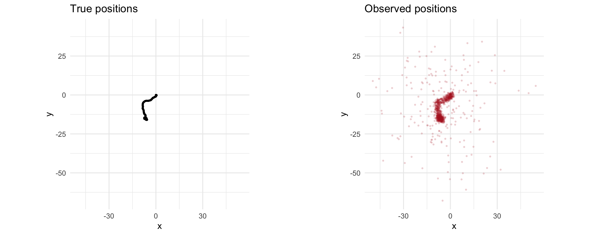

Kalman Filtering Recovery

The code below solves the standard Kalman filtering problem using CVXR. Note that the recovery is distorted by outliers in the measurements.

x <- Variable(c(4, N + 1))
w <- Variable(c(2, N))
v <- Variable(c(2, N))

tau <- 0.08

obj_kf <- sum_squares(w) + tau * sum_squares(v)
obj_kf <- Minimize(obj_kf)

constr <- list()
for (t in 1:N) {
    constr <- c(constr,
                list(x[, t + 1] == A %*% x[, t] + B %*% w[, t]),
                list(y[, t] == C %*% x[, t] + v[, t]))
}

prob_kf <- Problem(obj_kf, constr)
result_kf <- psolve(prob_kf, solver = "OSQP", verbose = TRUE)

────────────────────────────────── CVXR v1.8.1 ─────────────────────────────────

ℹ Problem: 3 variables, 2000 constraints (QP)

ℹ Compilation: "OSQP" via CVXR::Dcp2Cone -> CVXR::CvxAttr2Constr -> CVXR::ConeMatrixStuffing -> CVXR::OSQP_QP_Solver

ℹ Compile time: 8.518s

─────────────────────────────── Numerical solver ───────────────────────────────

-----------------------------------------------------------------
           OSQP v1.0.0  -  Operator Splitting QP Solver
              (c) The OSQP Developer Team
-----------------------------------------------------------------
problem:  variables n = 8004, constraints m = 6000
          nnz(P) + nnz(A) = 22000
settings: algebra = Built-in,
          OSQPInt = 4 bytes, OSQPFloat = 8 bytes,
          linear system solver = QDLDL v0.1.8,
          eps_abs = 1.0e-05, eps_rel = 1.0e-05,
          eps_prim_inf = 1.0e-04, eps_dual_inf = 1.0e-04,
          rho = 1.00e-01 (adaptive: 50 iterations),
          sigma = 1.00e-06, alpha = 1.60, max_iter = 10000
          check_termination: on (interval 25, duality gap: on),
          time_limit: 1.00e+10 sec,
          scaling: on (10 iterations), scaled_termination: off
          warm starting: on, polishing: on, 
iter   objective    prim res   dual res   gap        rel kkt    rho         time
   1   0.0000e+00   6.78e+01   6.78e+03  -2.92e+07   6.78e+03   1.00e-01    1.89e-03s
  50   1.2343e+04   3.62e-07   9.14e-08  -4.38e-04   3.62e-07   1.00e-01    7.85e-03s
plsh   1.2343e+04   3.55e-15   7.99e-15   3.64e-12   3.64e-12   --------    9.34e-03s

status:               solved
solution polishing:   successful
number of iterations: 50
optimal objective:    12343.3353
dual objective:       12343.3353
duality gap:          3.6380e-12
primal-dual integral: 2.9233e+07
run time:             9.34e-03s
optimal rho estimate: 7.77e-02

──────────────────────────────────── Summary ───────────────────────────────────

✔ Status: optimal

✔ Optimal value: 12343.3

ℹ Compile time: 8.518s

ℹ Solver time: 0.016s

check_solver_status(prob_kf)
cat("Optimal objective value:", result_kf, "\n")

Optimal objective value: 12343.34

x_kf <- value(x)
df_kf <- data.frame(x = x_kf[1, 1:N], y = x_kf[2, 1:N])

p1 <- ggplot(df_true, aes(x = x, y = y)) +
    geom_point(color = "black", alpha = 0.4, size = 0.5) +
    coord_fixed(xlim = xlims, ylim = ylims) +
    labs(title = "True positions") + theme_minimal()

p2 <- ggplot(df_kf, aes(x = x, y = y)) +
    geom_point(color = "steelblue", alpha = 0.4, size = 0.5) +
    coord_fixed(xlim = xlims, ylim = ylims) +
    labs(title = "Kalman filter recovery") + theme_minimal()

grid.arrange(p1, p2, ncol = 2)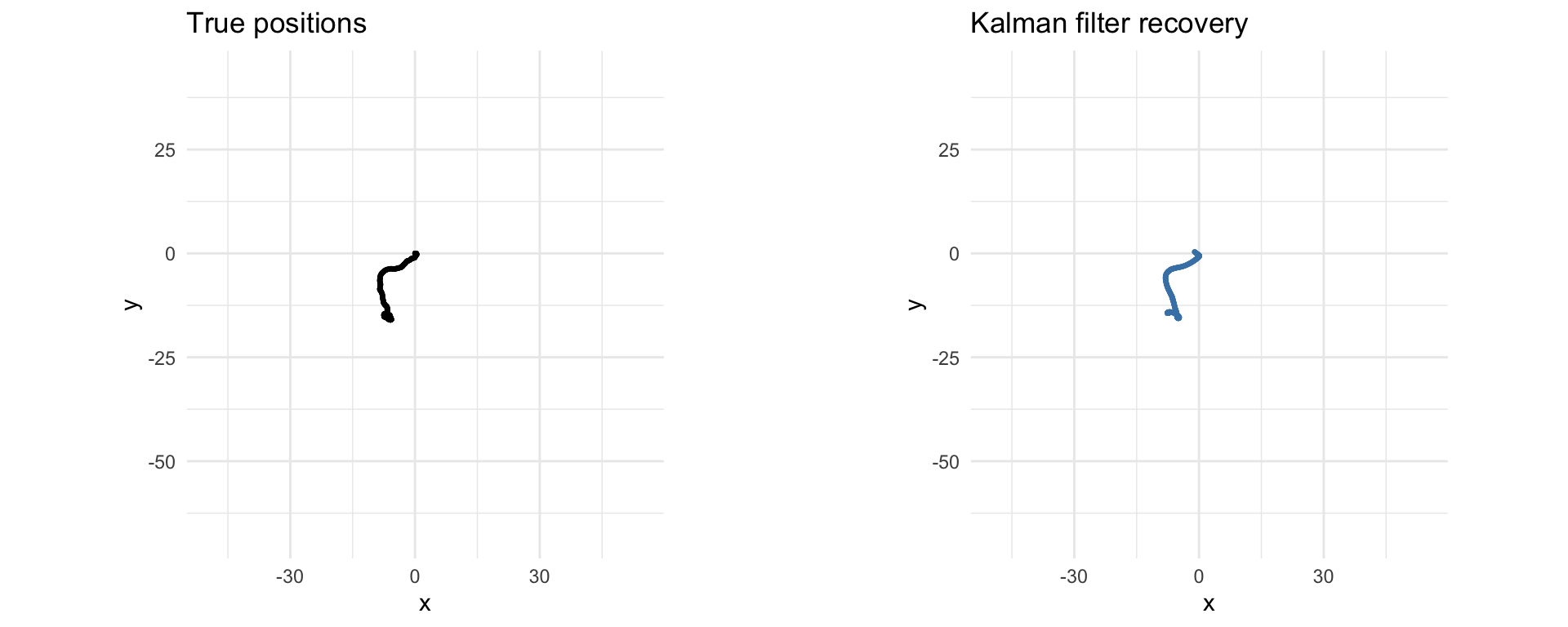

True and Kalman filter recovered positions

Robust Kalman Filtering Recovery

Here we implement robust Kalman filtering with CVXR, replacing the quadratic penalty on the noise with a Huber penalty. We get a better recovery than the standard Kalman filtering, as shown in the plots below.

x <- Variable(c(4, N + 1))
w <- Variable(c(2, N))
v <- Variable(c(2, N))

tau <- 2
rho <- 2

obj_rkf <- sum_squares(w)
huber_cost <- 0
for (t in 1:N) {
    huber_cost <- huber_cost + tau * huber(p_norm(v[, t], 2), rho)
}
obj_rkf <- Minimize(obj_rkf + huber_cost)

constr <- list()
for (t in 1:N) {
    constr <- c(constr,
                list(x[, t + 1] == A %*% x[, t] + B %*% w[, t]),
                list(y[, t] == C %*% x[, t] + v[, t]))
}

prob_rkf <- Problem(obj_rkf, constr)
result_rkf <- psolve(prob_rkf, solver = "SCS", verbose = TRUE)

────────────────────────────────── CVXR v1.8.1 ─────────────────────────────────

ℹ Problem: 3 variables, 2000 constraints (DCP)

ℹ Compilation: "SCS" via CVXR::Dcp2Cone -> CVXR::CvxAttr2Constr -> CVXR::ConeMatrixStuffing -> CVXR::SCS_Solver

ℹ Compile time: 22.09s

─────────────────────────────── Numerical solver ───────────────────────────────

------------------------------------------------------------------
           SCS v3.2.7 - Splitting Conic Solver
    (c) Brendan O'Donoghue, Stanford University, 2012
------------------------------------------------------------------
problem:  variables n: 12004, constraints m: 12000
cones:    z: primal zero / dual free vars: 7000
      l: linear vars: 2000
      q: soc vars: 3000, qsize: 1000
settings: eps_abs: 1.0e-05, eps_rel: 1.0e-05, eps_infeas: 1.0e-07
      alpha: 1.50, scale: 1.00e-01, adaptive_scale: 1
      max_iters: 100000, normalize: 1, rho_x: 1.00e-06
lin-sys:  sparse-direct-amd-qdldl
      nnz(A): 28000, nnz(P): 3000
------------------------------------------------------------------
 iter | pri res | dua res |   gap   |   obj   |  scale  | time (s)
------------------------------------------------------------------
     0| 1.13e+02  8.00e+00  9.36e+05 -4.37e+05  1.00e-01  6.21e-03 
   250| 1.01e-02  5.21e-04  1.14e+00  4.08e+04  1.00e-01  7.61e-02 
   375| 1.07e-03  2.96e-05  1.03e-01  4.08e+04  1.00e-01  1.11e-01 
------------------------------------------------------------------
status:  solved
timings: total: 1.11e-01s = setup: 5.40e-03s + solve: 1.05e-01s
     lin-sys: 8.15e-02s, cones: 5.90e-03s, accel: 0.00e+00s
------------------------------------------------------------------
objective = 40799.330860
------------------------------------------------------------------

──────────────────────────────────── Summary ───────────────────────────────────

✔ Status: optimal

✔ Optimal value: 40799.6

ℹ Compile time: 22.09s

ℹ Solver time: 0.117s

check_solver_status(prob_rkf)
cat("Optimal objective value:", result_rkf, "\n")

Optimal objective value: 40799.63

x_rkf <- value(x)
df_rkf <- data.frame(x = x_rkf[1, 1:N], y = x_rkf[2, 1:N])

p1 <- ggplot(df_true, aes(x = x, y = y)) +
    geom_point(color = "black", alpha = 0.4, size = 0.5) +
    coord_fixed(xlim = xlims, ylim = ylims) +
    labs(title = "True positions") + theme_minimal()

p2 <- ggplot(df_rkf, aes(x = x, y = y)) +
    geom_point(color = "darkgreen", alpha = 0.4, size = 0.5) +
    coord_fixed(xlim = xlims, ylim = ylims) +
    labs(title = "Robust Kalman filter recovery") + theme_minimal()

grid.arrange(p1, p2, ncol = 2)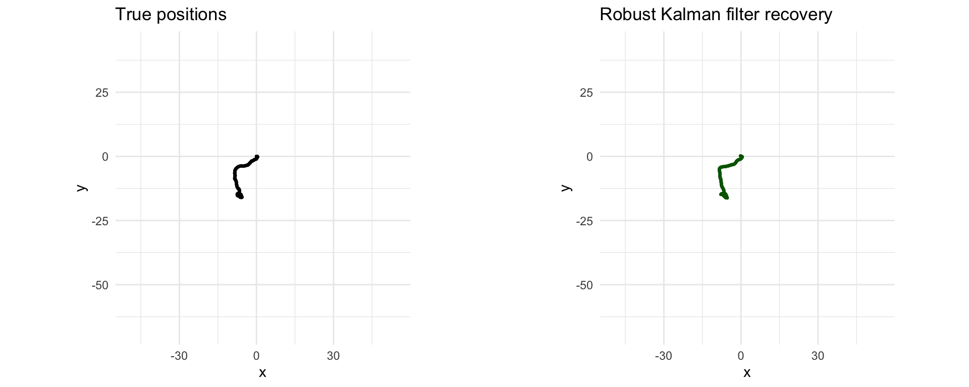

True and robust Kalman filter recovered positions

p1 <- ggplot(df_true, aes(x = x, y = y)) +
    geom_point(color = "black", alpha = 0.4, size = 0.5) +
    coord_fixed(xlim = xlims, ylim = ylims) +
    labs(title = "True") + theme_minimal()

p2 <- ggplot(df_obs, aes(x = x, y = y)) +
    geom_point(color = "firebrick", alpha = 0.15, size = 0.5) +
    coord_fixed(xlim = xlims, ylim = ylims) +
    labs(title = "Observed") + theme_minimal()

p3 <- ggplot(df_kf, aes(x = x, y = y)) +
    geom_point(color = "steelblue", alpha = 0.4, size = 0.5) +
    coord_fixed(xlim = xlims, ylim = ylims) +
    labs(title = "Kalman filter") + theme_minimal()

p4 <- ggplot(df_rkf, aes(x = x, y = y)) +
    geom_point(color = "darkgreen", alpha = 0.4, size = 0.5) +
    coord_fixed(xlim = xlims, ylim = ylims) +
    labs(title = "Robust Kalman filter") + theme_minimal()

grid.arrange(p1, p2, p3, p4, ncol = 2, nrow = 2)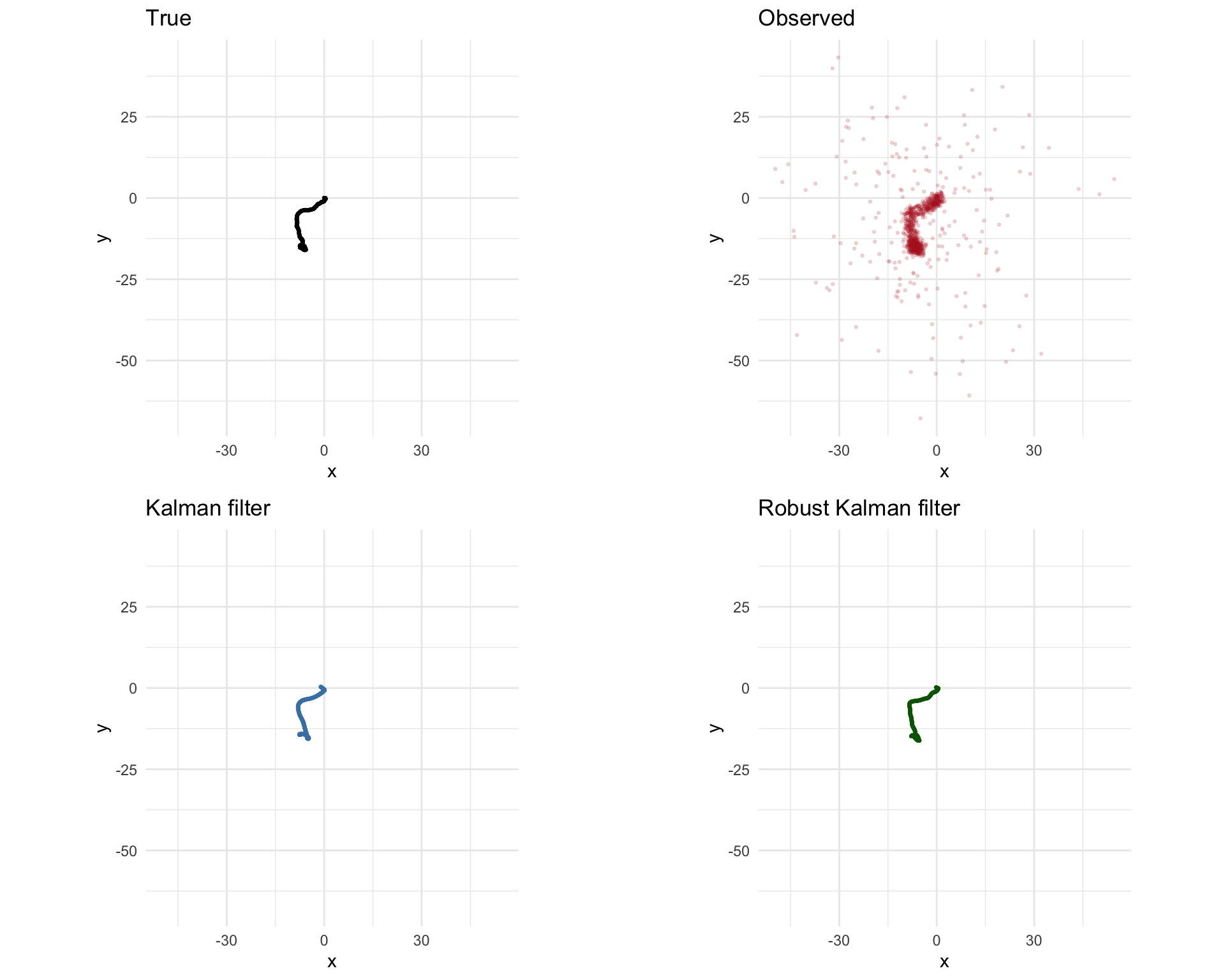

Comparison of all four position estimates

Session Info

R version 4.5.2 (2025-10-31)
Platform: aarch64-apple-darwin20
Running under: macOS Tahoe 26.3.1

Matrix products: default
BLAS:   /Library/Frameworks/R.framework/Versions/4.5-arm64/Resources/lib/libRblas.0.dylib 
LAPACK: /Library/Frameworks/R.framework/Versions/4.5-arm64/Resources/lib/libRlapack.dylib;  LAPACK version 3.12.1

locale:
[1] en_US.UTF-8/en_US.UTF-8/en_US.UTF-8/C/en_US.UTF-8/en_US.UTF-8

time zone: America/Los_Angeles
tzcode source: internal

attached base packages:
[1] stats     graphics  grDevices utils     datasets  methods   base     

other attached packages:
[1] gridExtra_2.3 ggplot2_4.0.2 CVXR_1.8.1   

loaded via a namespace (and not attached):
 [1] gmp_0.7-5.1        generics_0.1.4     clarabel_0.11.2    slam_0.1-55       
 [5] lattice_0.22-9     digest_0.6.39      magrittr_2.0.4     evaluate_1.0.5    
 [9] grid_4.5.2         RColorBrewer_1.1-3 fastmap_1.2.0      rprojroot_2.1.1   
[13] jsonlite_2.0.0     Matrix_1.7-4       ECOSolveR_0.6.1    backports_1.5.0   
[17] scs_3.2.7          Rmosek_11.1.1      scales_1.4.0       codetools_0.2-20  
[21] cli_3.6.5          rlang_1.1.7        Rglpk_0.6-5.1      withr_3.0.2       
[25] yaml_2.3.12        otel_0.2.0         tools_4.5.2        osqp_1.0.0        
[29] Rcplex_0.3-8       checkmate_2.3.4    dplyr_1.2.0        here_1.0.2        
[33] gurobi_13.0-1      vctrs_0.7.1        R6_2.6.1           lifecycle_1.0.5   
[37] htmlwidgets_1.6.4  pkgconfig_2.0.3    cccp_0.3-3         pillar_1.11.1     
[41] gtable_0.3.6       glue_1.8.0         Rcpp_1.1.1         xfun_0.56         
[45] tibble_3.3.1       tidyselect_1.2.1   knitr_1.51         dichromat_2.0-0.1 
[49] highs_1.12.0-3     farver_2.1.2       htmltools_0.5.9    labeling_0.4.3    
[53] rmarkdown_2.30     piqp_0.6.2         compiler_4.5.2     S7_0.2.1