Total Variation In-Painting

Author

CVXPY Developers and Balasubramanian Narasimhan

Introduction

A grayscale image is represented as an $m \times n$ matrix of intensities $U^{orig}$ (typically between the values $0$ and $255$ ). We are given the values $U_{i j}^{orig}$ , for $(i, j) \in K$ , where $K \subset {1, \dots, m} \times {1, \dots, n}$ is the set of indices corresponding to known pixel values. Our job is to in-paint the image by guessing the missing pixel values, i.e., those with indices not in $K$ . The reconstructed image will be represented by $U \in R^{m \times n}$ , where $U$ matches the known pixels, i.e., $U_{i j} = U_{i j}^{orig}$ for $(i, j) \in K$ .

The reconstruction $U$ is found by minimizing the total variation of $U$ , subject to matching the known pixel values. We use the $ℓ_{2}$ total variation, defined as

$t v (U) = \sum_{i = 1}^{m - 1} \sum_{j = 1}^{n - 1} {‖ (\begin{matrix} U_{i + 1, j} - U_{i j} \\ U_{i, j + 1} - U_{i j} \end{matrix}) ‖}_{2} .$

Note that the norm of the discretized gradient is not squared.

Grayscale In-Painting

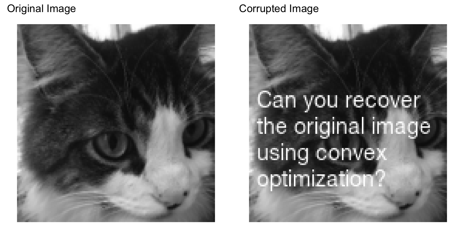
We load a $128 \times 128$ grayscale image and a corrupted version where text has been overlaid on the original. The corrupted image has white text obscuring parts of the image. We construct the known matrix by comparing the two images: a pixel is known if it was not affected by the text overlay.

## Load the images
u_orig <- readPNG(here::here("images", "loki128.png"))
u_corr <- readPNG(here::here("images", "loki128_corrupted.png"))

## If images are RGB, convert to grayscale by averaging channels
if (length(dim(u_orig)) == 3) {
    u_orig <- (u_orig[, , 1] + u_orig[, , 2] + u_orig[, , 3]) / 3
}
if (length(dim(u_corr)) == 3) {
    u_corr <- (u_corr[, , 1] + u_corr[, , 2] + u_corr[, , 3]) / 3
}

rows <- nrow(u_orig)
cols <- ncol(u_orig)

## known is 1 if the pixel is known, 0 if corrupted
known <- 1 * (u_orig == u_corr)
cat("Image size:", rows, "x", cols, "\n")
cat("Known pixels:", sum(known), "out of", rows * cols,
    sprintf("(%.0f%%)\n", 100 * sum(known) / (rows * cols)))

Image size: 128 x 128 
Known pixels: 14090 out of 16384 (86%)

p1 <- ggplot() +
    annotation_raster(matrix(gray(u_orig), rows, cols),
                      xmin = 0, xmax = 1, ymin = 0, ymax = 1,
                      interpolate = FALSE) +
    coord_fixed() + theme_void() + ggtitle("Original Image")

p2 <- ggplot() +
    annotation_raster(matrix(gray(u_corr), rows, cols),
                      xmin = 0, xmax = 1, ymin = 0, ymax = 1,
                      interpolate = FALSE) +
    coord_fixed() + theme_void() + ggtitle("Corrupted Image")

grid.arrange(p1, p2, ncol = 2)

Original (left) and corrupted (right) grayscale images

Now we solve the total variation in-painting problem using CVXR. We use the SCS solver, which scales well to larger problems.

U <- Variable(c(rows, cols))
obj <- Minimize(tv(U))

Warning: `tv()` is deprecated. Use `total_variation()` instead.
This warning is displayed once per session.

constraints <- list(multiply(known, U) == multiply(known, u_corr))

Warning: `multiply()` is deprecated. Use `x * y` instead.
This warning is displayed once per session.

prob <- Problem(obj, constraints)

result <- psolve(prob, solver = "SCS", verbose = TRUE)

────────────────────────────────── CVXR v1.8.1 ─────────────────────────────────

ℹ Problem: 1 variable, 1 constraint (DCP)

ℹ Compilation: "SCS" via CVXR::Dcp2Cone -> CVXR::CvxAttr2Constr -> CVXR::ConeMatrixStuffing -> CVXR::SCS_Solver

ℹ Compile time: 0.511s

─────────────────────────────── Numerical solver ───────────────────────────────

------------------------------------------------------------------
           SCS v3.2.7 - Splitting Conic Solver
    (c) Brendan O'Donoghue, Stanford University, 2012
------------------------------------------------------------------
problem:  variables n: 32513, constraints m: 64771
cones:    z: primal zero / dual free vars: 16384
      q: soc vars: 48387, qsize: 16129
settings: eps_abs: 1.0e-05, eps_rel: 1.0e-05, eps_infeas: 1.0e-07
      alpha: 1.50, scale: 1.00e-01, adaptive_scale: 1
      max_iters: 100000, normalize: 1, rho_x: 1.00e-06
lin-sys:  sparse-direct-amd-qdldl
      nnz(A): 94735, nnz(P): 0
------------------------------------------------------------------
 iter | pri res | dua res |   gap   |   obj   |  scale  | time (s)
------------------------------------------------------------------
     0| 2.55e+01  1.00e+00  4.12e+05 -2.06e+05  1.00e-01  3.62e-02 
   250| 3.67e-02  3.19e-03  2.14e-03  7.02e+02  1.00e-01  4.96e-01 
   500| 7.86e-03  1.17e-03  2.29e-04  7.39e+02  3.18e-01  9.68e-01 
   750| 3.92e-03  2.40e-04  1.29e-04  7.40e+02  3.18e-01  1.42e+00 
  1000| 2.92e-03  3.02e-04  9.42e-06  7.40e+02  3.18e-01  1.87e+00 
  1250| 1.64e-03  5.45e-04  1.47e-05  7.40e+02  1.01e+00  2.33e+00 
  1500| 6.00e-04  5.97e-05  3.85e-06  7.40e+02  1.01e+00  2.77e+00 
  1750| 3.25e-04  1.16e-04  8.73e-07  7.40e+02  1.01e+00  3.22e+00 
  2000| 2.52e-04  2.20e-05  2.38e-07  7.40e+02  1.01e+00  3.67e+00 
  2250| 2.17e-04  1.59e-06  2.76e-07  7.40e+02  1.01e+00  4.12e+00 
  2500| 1.34e-04  4.88e-05  1.71e-06  7.40e+02  3.28e+00  4.57e+00 
  2750| 8.74e-05  4.66e-06  3.22e-07  7.40e+02  3.28e+00  5.02e+00 
  3000| 7.06e-05  2.88e-06  1.51e-08  7.40e+02  3.28e+00  5.47e+00 
  3250| 6.30e-05  1.95e-06  2.57e-07  7.40e+02  3.28e+00  5.92e+00 
  3500| 3.37e-05  2.03e-04  1.36e-06  7.40e+02  1.04e+01  6.37e+00 
  3750| 2.56e-05  8.62e-05  1.08e-06  7.40e+02  1.04e+01  6.82e+00 
  3850| 1.77e-05  3.97e-06  8.25e-07  7.40e+02  1.04e+01  7.00e+00 
------------------------------------------------------------------
status:  solved
timings: total: 7.00e+00s = setup: 3.29e-02s + solve: 6.97e+00s
     lin-sys: 5.06e+00s, cones: 8.29e-01s, accel: 0.00e+00s
------------------------------------------------------------------
objective = 740.137245
------------------------------------------------------------------

──────────────────────────────────── Summary ───────────────────────────────────

✔ Status: optimal

✔ Optimal value: 740.137

ℹ Compile time: 0.511s

ℹ Solver time: 7.009s

check_solver_status(prob)
cat("Optimal objective value:", result, "\n")

Optimal objective value: 740.1374

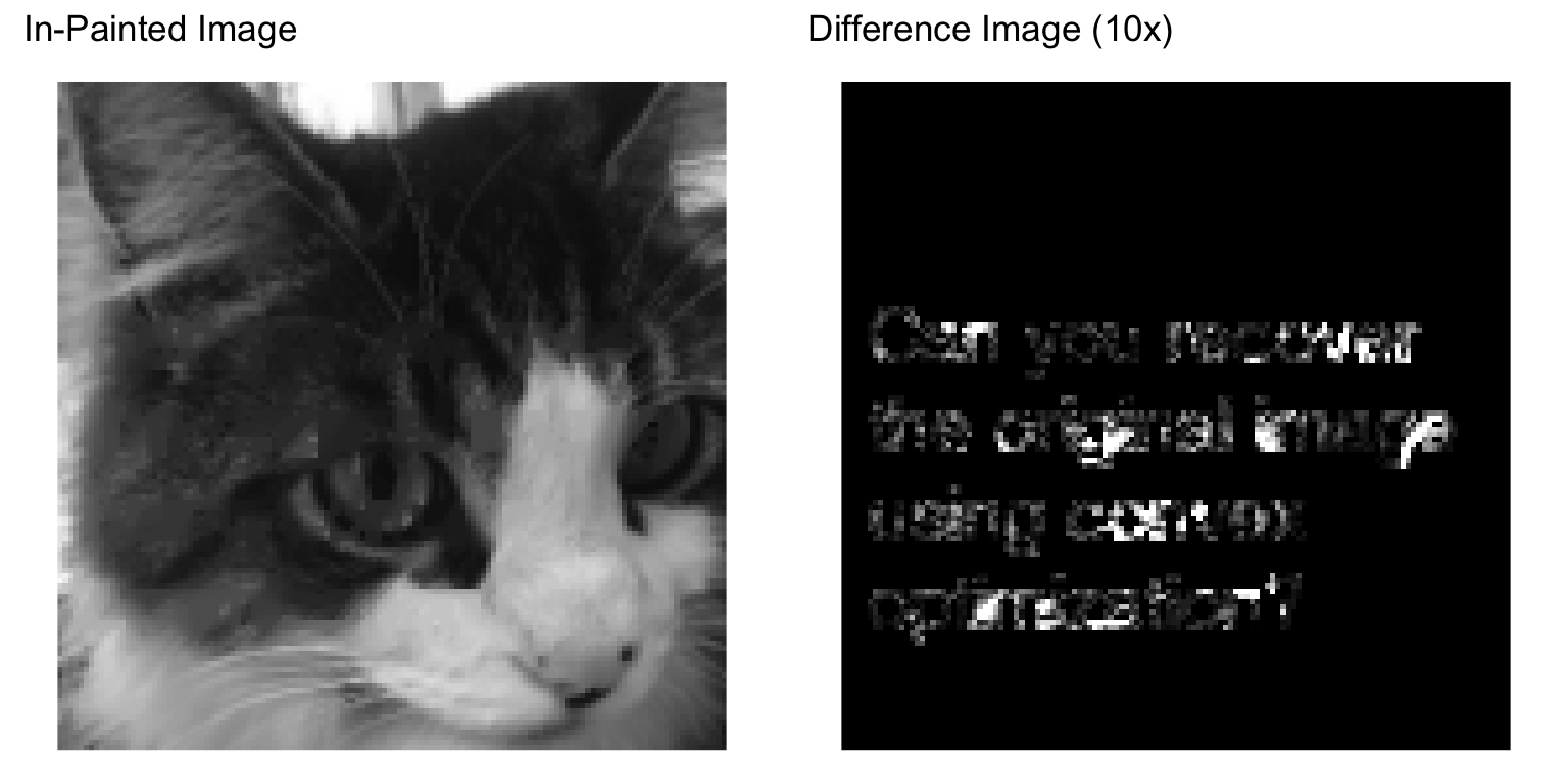
After solving the problem, the in-painted image is stored in the value of U. We display the in-painted image and the intensity difference between the original and in-painted images (magnified by a factor of 10 for visibility).

U_val <- pmin(pmax(value(U), 0), 1)

p3 <- ggplot() +
    annotation_raster(matrix(gray(U_val), rows, cols),
                      xmin = 0, xmax = 1, ymin = 0, ymax = 1,
                      interpolate = FALSE) +
    coord_fixed() + theme_void() + ggtitle("In-Painted Image")

img_diff <- pmin(10 * abs(u_orig - U_val), 1)
p4 <- ggplot() +
    annotation_raster(matrix(gray(img_diff), rows, cols),
                      xmin = 0, xmax = 1, ymin = 0, ymax = 1,
                      interpolate = FALSE) +
    coord_fixed() + theme_void() + ggtitle("Difference Image (10x)")

grid.arrange(p3, p4, ncol = 2)

In-painted (left) and difference (right) grayscale images

Color In-Painting

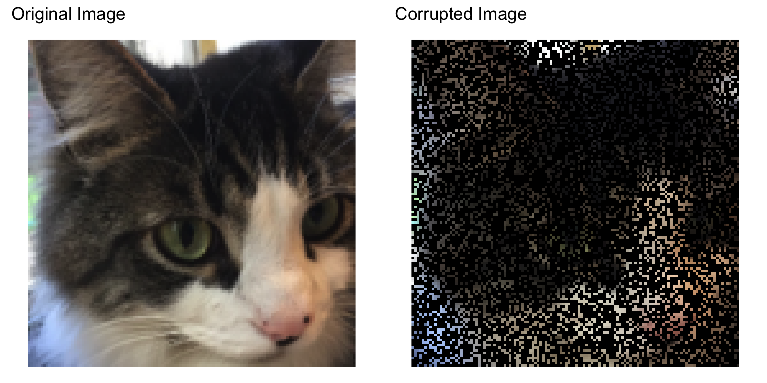
For color images, the in-painting problem is similar to the grayscale case. A color image is represented as an $m \times n \times 3$ array of RGB values $U^{orig}$ (typically between the values $0$ and $1$ ). We solve the problem by creating three CVXR variables (one per color channel) and minimizing the total variation jointly across all channels.

We load a $128 \times 128$ color image and randomly discard $70 %$ of the pixels.

set.seed(1)

## Load color image
u_orig_color <- readPNG(here::here("images", "loki128color.png"))
## Drop alpha channel if present
if (dim(u_orig_color)[3] == 4) {
    u_orig_color <- u_orig_color[, , 1:3]
}
rows_c <- dim(u_orig_color)[1]
cols_c <- dim(u_orig_color)[2]
colors <- dim(u_orig_color)[3]

## known is 1 if the pixel is known, 0 if corrupted
## Randomly keep 30% of pixels
pixel_mask <- matrix(as.numeric(runif(rows_c * cols_c) > 0.7), rows_c, cols_c)
known_color <- array(rep(pixel_mask, colors), dim = c(rows_c, cols_c, colors))

u_corr_color <- known_color * u_orig_color
cat("Color image size:", rows_c, "x", cols_c, "x", colors, "\n")

Color image size: 128 x 128 x 3

## Helper to convert array to raster string matrix for ggplot
arr_to_raster <- function(arr) {
    arr <- pmin(pmax(arr, 0), 1)
    nr <- dim(arr)[1]; nc <- dim(arr)[2]
    matrix(rgb(arr[, , 1], arr[, , 2], arr[, , 3]), nr, nc)
}

p5 <- ggplot() +
    annotation_raster(arr_to_raster(u_orig_color),
                      xmin = 0, xmax = 1, ymin = 0, ymax = 1,
                      interpolate = FALSE) +
    coord_fixed() + theme_void() + ggtitle("Original Image")

p6 <- ggplot() +
    annotation_raster(arr_to_raster(u_corr_color),
                      xmin = 0, xmax = 1, ymin = 0, ymax = 1,
                      interpolate = FALSE) +
    coord_fixed() + theme_void() + ggtitle("Corrupted Image")

grid.arrange(p5, p6, ncol = 2)

Original (left) and corrupted (right) color images

## Solve the TV in-painting problem for each channel
channels <- lapply(seq_len(colors), function(k) {
    U_k <- Variable(c(rows_c, cols_c))
    constr <- multiply(known_color[, , k], U_k) ==
              multiply(known_color[, , k], u_corr_color[, , k])
    list(var = U_k, constr = constr)
})
variables <- lapply(channels, `[[`, "var")
constraints_c <- lapply(channels, `[[`, "constr")

prob_color <- Problem(Minimize(tv(variables[[1]], variables[[2]], variables[[3]])),
                      constraints_c)
result_color <- psolve(prob_color, solver = "SCS", verbose = TRUE)

────────────────────────────────── CVXR v1.8.1 ─────────────────────────────────

ℹ Problem: 3 variables, 3 constraints (DCP)

ℹ Compilation: "SCS" via CVXR::Dcp2Cone -> CVXR::CvxAttr2Constr -> CVXR::ConeMatrixStuffing -> CVXR::SCS_Solver

ℹ Compile time: 0.185s

─────────────────────────────── Numerical solver ───────────────────────────────

------------------------------------------------------------------
           SCS v3.2.7 - Splitting Conic Solver
    (c) Brendan O'Donoghue, Stanford University, 2012
------------------------------------------------------------------
problem:  variables n: 65281, constraints m: 162055
cones:    z: primal zero / dual free vars: 49152
      q: soc vars: 112903, qsize: 16129
settings: eps_abs: 1.0e-05, eps_rel: 1.0e-05, eps_infeas: 1.0e-07
      alpha: 1.50, scale: 1.00e-01, adaptive_scale: 1
      max_iters: 100000, normalize: 1, rho_x: 1.00e-06
lin-sys:  sparse-direct-amd-qdldl
      nnz(A): 224494, nnz(P): 0
------------------------------------------------------------------
 iter | pri res | dua res |   gap   |   obj   |  scale  | time (s)
------------------------------------------------------------------
     0| 2.71e+01  1.00e+00  4.37e+05 -2.19e+05  1.00e-01  1.01e-01 
   250| 3.78e-02  1.89e-03  1.93e-03  9.35e+02  1.00e-01  1.25e+00 
   500| 8.36e-03  1.64e-03  4.75e-04  9.66e+02  3.22e-01  2.43e+00 
   750| 4.67e-03  7.06e-04  1.28e-04  9.68e+02  3.22e-01  3.57e+00 
  1000| 2.71e-03  1.89e-04  5.94e-05  9.68e+02  3.22e-01  4.71e+00 
  1250| 1.80e-03  1.08e-04  3.16e-05  9.68e+02  3.22e-01  5.84e+00 
  1500| 1.38e-03  1.19e-04  2.03e-05  9.68e+02  3.22e-01  6.98e+00 
  1750| 1.14e-03  8.68e-05  1.45e-05  9.68e+02  3.22e-01  8.11e+00 
  2000| 1.06e-03  1.20e-04  2.89e-05  9.68e+02  1.02e+00  9.27e+00 
  2250| 4.84e-04  6.17e-05  1.28e-05  9.68e+02  1.02e+00  1.04e+01 
  2500| 4.15e-04  3.26e-05  7.78e-06  9.68e+02  1.02e+00  1.15e+01 
  2750| 2.30e-04  1.39e-05  5.35e-06  9.68e+02  1.02e+00  1.27e+01 
  3000| 1.61e-04  1.98e-06  4.37e-06  9.68e+02  1.02e+00  1.38e+01 
  3250| 1.23e-04  1.84e-05  3.47e-06  9.68e+02  1.02e+00  1.49e+01 
  3500| 1.07e-04  8.27e-05  1.95e-06  9.68e+02  3.25e+00  1.61e+01 
  3750| 6.34e-05  2.19e-06  4.58e-07  9.68e+02  3.25e+00  1.72e+01 
  4000| 5.02e-05  1.54e-06  1.16e-07  9.68e+02  3.25e+00  1.83e+01 
  4250| 4.36e-05  2.85e-06  4.55e-07  9.68e+02  3.25e+00  1.95e+01 
  4500| 3.97e-05  2.16e-06  6.45e-07  9.68e+02  3.25e+00  2.06e+01 
  4625| 1.83e-05  1.45e-05  2.70e-06  9.68e+02  1.03e+01  2.12e+01 
------------------------------------------------------------------
status:  solved
timings: total: 2.12e+01s = setup: 9.21e-02s + solve: 2.11e+01s
     lin-sys: 1.62e+01s, cones: 1.85e+00s, accel: 0.00e+00s
------------------------------------------------------------------
objective = 968.179779
------------------------------------------------------------------

──────────────────────────────────── Summary ───────────────────────────────────

✔ Status: optimal

✔ Optimal value: 968.181

ℹ Compile time: 0.185s

ℹ Solver time: 21.213s

check_solver_status(prob_color)
cat("Optimal objective value:", result_color, "\n")

Optimal objective value: 968.1805

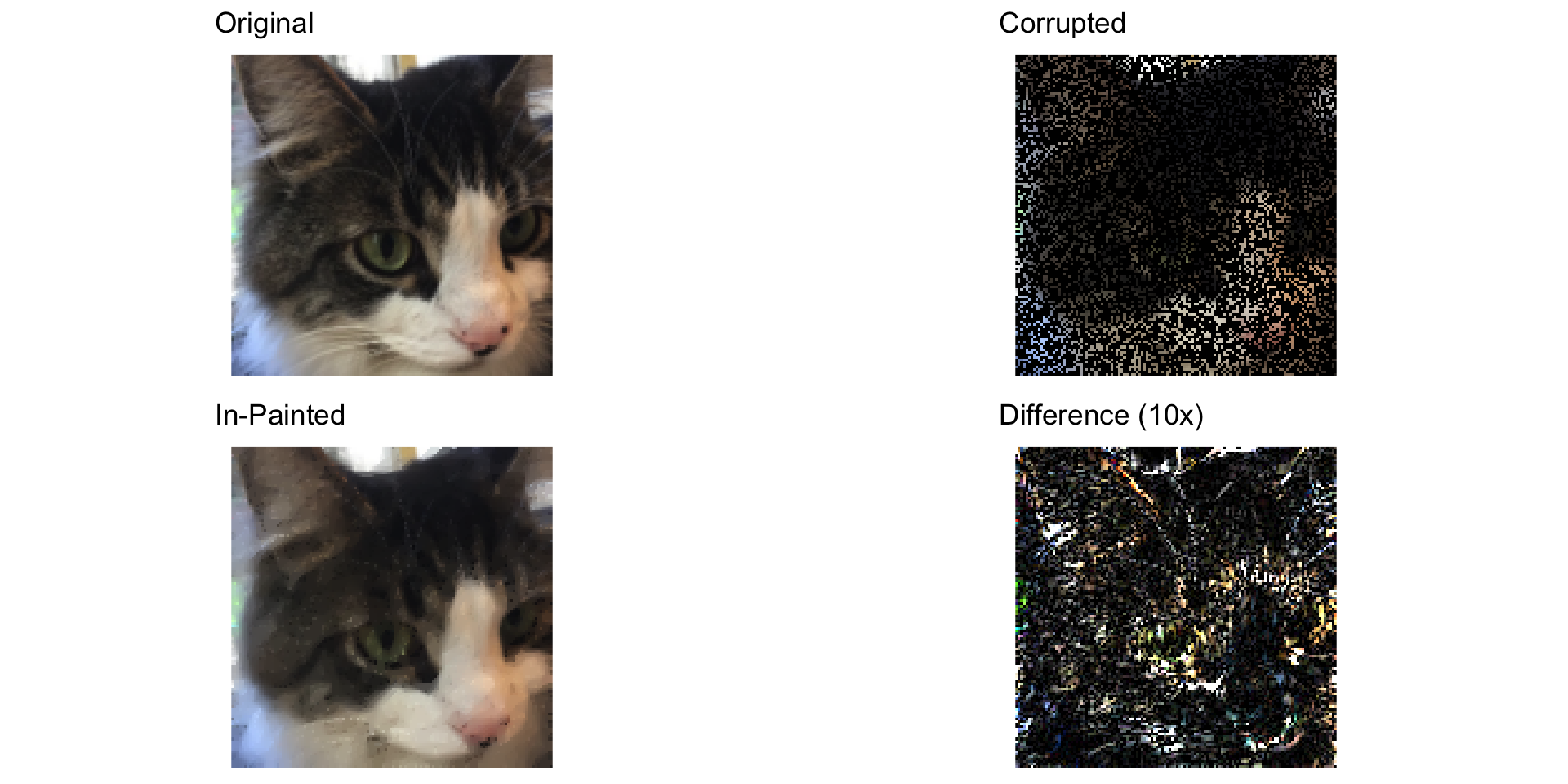
After solving, we reconstruct the color image and compare with the original.

rec_arr <- array(
    unlist(lapply(variables, function(v) pmin(pmax(value(v), 0), 1))),
    dim = c(rows_c, cols_c, colors)
)

p7 <- ggplot() +
    annotation_raster(arr_to_raster(u_orig_color),
                      xmin = 0, xmax = 1, ymin = 0, ymax = 1,
                      interpolate = FALSE) +
    coord_fixed() + theme_void() + ggtitle("Original")

p8 <- ggplot() +
    annotation_raster(arr_to_raster(u_corr_color),
                      xmin = 0, xmax = 1, ymin = 0, ymax = 1,
                      interpolate = FALSE) +
    coord_fixed() + theme_void() + ggtitle("Corrupted")

p9 <- ggplot() +
    annotation_raster(arr_to_raster(rec_arr),
                      xmin = 0, xmax = 1, ymin = 0, ymax = 1,
                      interpolate = FALSE) +
    coord_fixed() + theme_void() + ggtitle("In-Painted")

diff_arr <- pmin(10 * abs(u_orig_color - rec_arr), 1)
p10 <- ggplot() +
    annotation_raster(arr_to_raster(diff_arr),
                      xmin = 0, xmax = 1, ymin = 0, ymax = 1,
                      interpolate = FALSE) +
    coord_fixed() + theme_void() + ggtitle("Difference (10x)")

grid.arrange(p7, p8, p9, p10, ncol = 2)

Original, corrupted, in-painted, and difference color images

Session Info

R version 4.5.2 (2025-10-31)
Platform: aarch64-apple-darwin20
Running under: macOS Tahoe 26.3

Matrix products: default
BLAS:   /Library/Frameworks/R.framework/Versions/4.5-arm64/Resources/lib/libRblas.0.dylib 
LAPACK: /Library/Frameworks/R.framework/Versions/4.5-arm64/Resources/lib/libRlapack.dylib;  LAPACK version 3.12.1

locale:
[1] en_US.UTF-8/en_US.UTF-8/en_US.UTF-8/C/en_US.UTF-8/en_US.UTF-8

time zone: America/Los_Angeles
tzcode source: internal

attached base packages:
[1] grid      stats     graphics  grDevices utils     datasets  methods  
[8] base     

other attached packages:
[1] gridExtra_2.3 ggplot2_4.0.2 png_0.1-8     CVXR_1.8.1   

loaded via a namespace (and not attached):
 [1] gmp_0.7-5.1        generics_0.1.4     clarabel_0.11.2    slam_0.1-55       
 [5] lattice_0.22-9     digest_0.6.39      magrittr_2.0.4     evaluate_1.0.5    
 [9] RColorBrewer_1.1-3 fastmap_1.2.0      rprojroot_2.1.1    jsonlite_2.0.0    
[13] Matrix_1.7-4       ECOSolveR_0.6.1    backports_1.5.0    scs_3.2.7         
[17] Rmosek_11.1.1      scales_1.4.0       codetools_0.2-20   cli_3.6.5         
[21] rlang_1.1.7        Rglpk_0.6-5.1      withr_3.0.2        yaml_2.3.12       
[25] otel_0.2.0         tools_4.5.2        osqp_1.0.0         Rcplex_0.3-8      
[29] checkmate_2.3.4    dplyr_1.2.0        here_1.0.2         gurobi_13.0-1     
[33] vctrs_0.7.1        R6_2.6.1           lifecycle_1.0.5    htmlwidgets_1.6.4 
[37] pkgconfig_2.0.3    cccp_0.3-3         pillar_1.11.1      gtable_0.3.6      
[41] glue_1.8.0         Rcpp_1.1.1         xfun_0.56          tibble_3.3.1      
[45] tidyselect_1.2.1   knitr_1.51         dichromat_2.0-0.1  highs_1.12.0-3    
[49] farver_2.1.2       htmltools_0.5.9    rmarkdown_2.30     piqp_0.6.2        
[53] compiler_4.5.2     S7_0.2.1

Introduction

Grayscale In-Painting

Color In-Painting

Session Info

References