Chebyshev Design of an FIR Filter

Author

CVXPY Developers and Balasubramanian Narasimhan

Introduction

This example is adapted from the CVX example of the same name, by Almir Mutapcic (2/2/2006) and the CVXPY adaptation by Judson Wilson (5/27/2014).

This program designs an FIR filter, given a desired frequency response $H_{des} (ω)$ . The design is judged by the maximum absolute error (Chebyshev norm). This is a convex problem (after sampling it can be formulated as an SOCP), which may be written in the form:

$\begin{array}{ll} minimize & max | H (ω) - H_{des} (ω) | for 0 \leq ω \leq π, \end{array}$

where the variable $H$ is the frequency response function, corresponding to an impulse response $h$ .

Topic reference: “Filter design” lecture notes (EE364) by S. Boyd.

Problem Data

## Number of FIR coefficients (including the zeroth one)
n <- 20

## Rule-of-thumb frequency discretization (Cheney's Approx. Theory book)
m <- 15 * n
w <- seq(0, pi, length.out = m)

## Construct the desired filter: fractional delay
D <- 8.25              # Delay value
Hdes <- exp(-1i * D * w)  # Desired frequency response

Solve the Minimax (Chebyshev) Design Problem

The frequency response from a vector of filter coefficients $h$ is computed as $H (ω) = \sum_{k = 0}^{n - 1} h_{k} e^{- j k ω}$ , which can be expressed in matrix form as $H = A h$ where $A_{ω, k} = e^{- j k ω}$ .

Since CVXR works with real-valued math, we split the problem into real and imaginary parts. The objective becomes:

$minimize max_{ω} [(Re (A) h - Re (H_{des}))^{2} + (Im (A) h - Im (H_{des}))^{2}] .$

## A is the matrix used to compute the frequency response
## A[w,:] = [1, exp(-j*w), exp(-j*2*w), ..., exp(-j*(n-1)*w)]
A <- exp(-1i * outer(w, 0:(n-1)))

## Split into real and imaginary parts
Hdes_r <- Re(Hdes)
Hdes_i <- Im(Hdes)
A_R <- Re(A)
A_I <- Im(A)

## h is the (real) FIR coefficient vector
h <- Variable(n)

## The objective minimizes max(|A*h - Hdes|^2)
## = max( (Re(A)*h - Re(Hdes))^2 + (Im(A)*h - Im(Hdes))^2 )
obj <- Minimize(
    max_entries(
        (A_R %*% h - Hdes_r)^2 + (A_I %*% h - Hdes_i)^2
    )
)

## Solve problem
prob <- Problem(obj)
result <- psolve(prob)

cat(sprintf("Problem status: %s\n", status(prob)))
cat(sprintf("Final objective value: %f\n", result))

Problem status: optimal
Final objective value: 0.500000

Result Plots

We plot the FIR impulse response, and the frequency response magnitude and phase.

h_val <- value(h)
df_impulse <- data.frame(n = 0:(n-1), h = as.numeric(h_val))

ggplot(df_impulse, aes(x = n, y = h)) +
    geom_segment(aes(xend = n, yend = 0)) +
    geom_point() +
    labs(x = "n", y = "h(n)", title = "FIR Filter Impulse Response") +
    theme_minimal()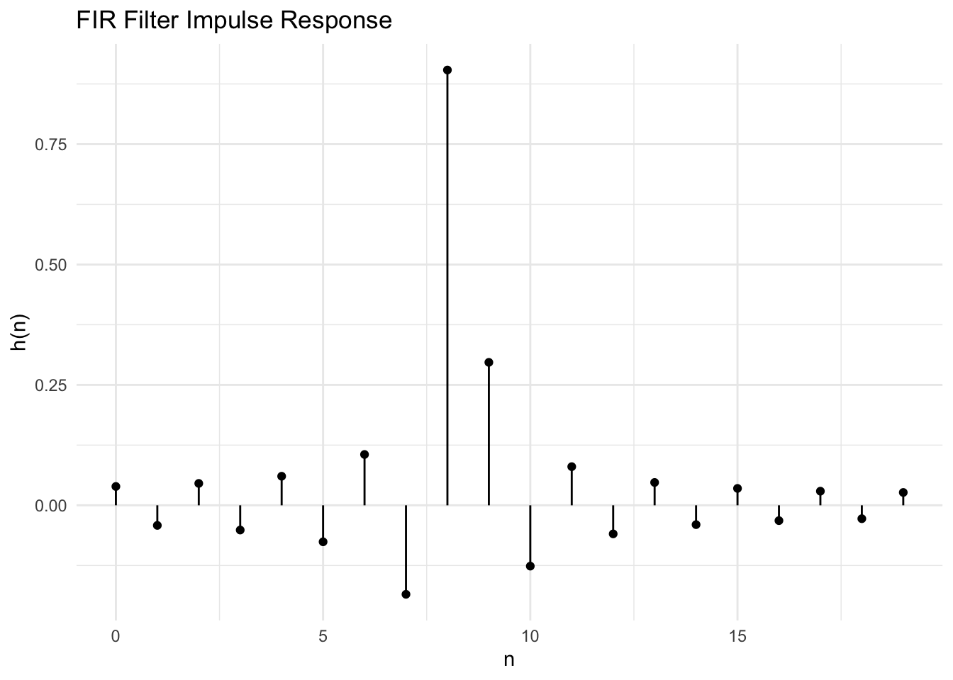

## Compute the frequency response
H <- as.vector(A %*% h_val)

df_mag <- data.frame(
    omega = rep(w, 2),
    magnitude = c(20 * log10(Mod(H)), 20 * log10(Mod(Hdes))),
    type = rep(c("Optimized", "Desired"), each = m)
)

ggplot(df_mag, aes(x = omega, y = magnitude, color = type, linetype = type)) +
    geom_line() +
    scale_linetype_manual(values = c("Desired" = "dashed", "Optimized" = "solid")) +
    coord_cartesian(xlim = c(0, pi), ylim = c(-30, 10)) +
    labs(x = expression(omega), y = expression(paste("|H(", omega, ")| in dB")),
         title = "FIR Filter Frequency Response Magnitude",
         color = "", linetype = "") +
    theme_minimal() +
    theme(legend.position = "bottom")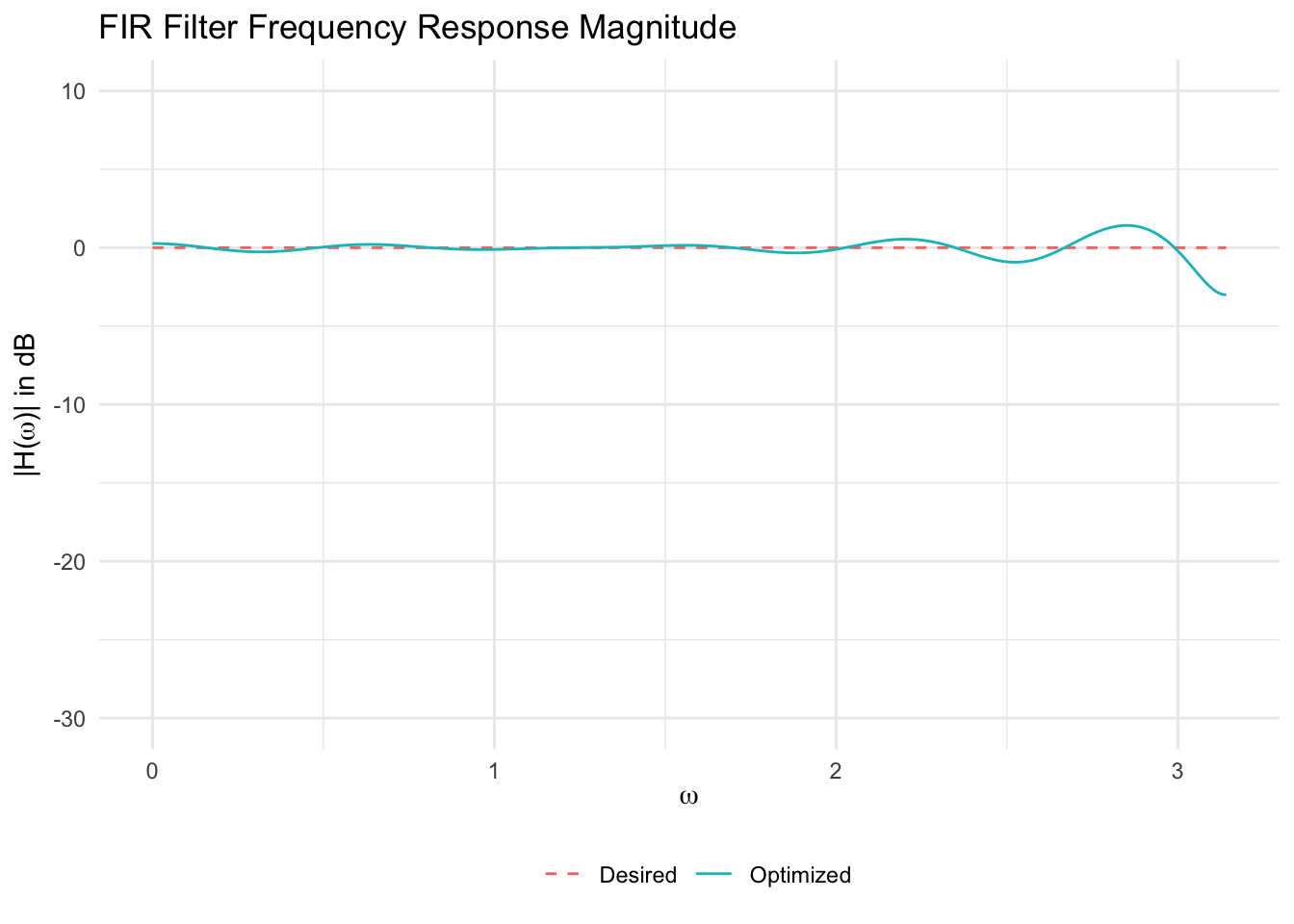

df_phase <- data.frame(omega = w, phase = Arg(H))

ggplot(df_phase, aes(x = omega, y = phase)) +
    geom_line() +
    coord_cartesian(xlim = c(0, pi), ylim = c(-pi, pi)) +
    labs(x = expression(omega), y = expression(paste(symbol("\xd0"), " H(", omega, ")")),
         title = "FIR Filter Frequency Response Phase") +
    theme_minimal()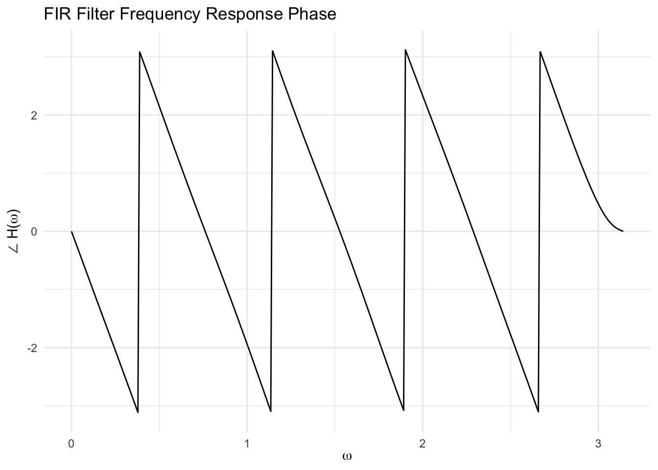

Session Info

R version 4.5.2 (2025-10-31)
Platform: aarch64-apple-darwin20
Running under: macOS Tahoe 26.3

Matrix products: default
BLAS:   /Library/Frameworks/R.framework/Versions/4.5-arm64/Resources/lib/libRblas.0.dylib 
LAPACK: /Library/Frameworks/R.framework/Versions/4.5-arm64/Resources/lib/libRlapack.dylib;  LAPACK version 3.12.1

locale:
[1] en_US.UTF-8/en_US.UTF-8/en_US.UTF-8/C/en_US.UTF-8/en_US.UTF-8

time zone: America/Los_Angeles
tzcode source: internal

attached base packages:
[1] stats     graphics  grDevices datasets  utils     methods   base     

other attached packages:
[1] ggplot2_4.0.2   CVXR_1.8.0.9213

loaded via a namespace (and not attached):
 [1] piqp_0.6.2         Matrix_1.7-4       gtable_0.3.6       jsonlite_2.0.0    
 [5] dplyr_1.2.0        compiler_4.5.2     highs_1.12.0-3     tidyselect_1.2.1  
 [9] Rcpp_1.1.1         slam_0.1-55        cccp_0.3-3         dichromat_2.0-0.1 
[13] scales_1.4.0       yaml_2.3.12        fastmap_1.2.0      clarabel_0.11.2   
[17] lattice_0.22-9     R6_2.6.1           labeling_0.4.3     generics_0.1.4    
[21] knitr_1.51         htmlwidgets_1.6.4  backports_1.5.0    Rcplex_0.3-8      
[25] gurobi_13.0-1      checkmate_2.3.4    tibble_3.3.1       osqp_1.0.0        
[29] pillar_1.11.1      RColorBrewer_1.1-3 rlang_1.1.7        xfun_0.56         
[33] S7_0.2.1           otel_0.2.0         cli_3.6.5          withr_3.0.2       
[37] magrittr_2.0.4     Rglpk_0.6-5.1      digest_0.6.39      grid_4.5.2        
[41] gmp_0.7-5.1        lifecycle_1.0.5    ECOSolveR_0.6.1    scs_3.2.7         
[45] vctrs_0.7.1        evaluate_1.0.5     glue_1.8.0         farver_2.1.2      
[49] codetools_0.2-20   Rmosek_11.1.1      rmarkdown_2.30     pkgconfig_2.0.3   
[53] tools_4.5.2        htmltools_0.5.9

References

Boyd, S. “Filter design” lecture notes (EE364), Stanford University.
Mutapcic, A. (2006). CVX example: Chebyshev design of an FIR filter.