library(devtools)
install_github("hadley/l1tf")L1 Trend Filtering
Introduction
Kim et al. (2009) propose the \(l_1\) trend filtering method for trend estimation. The method solves an optimization problem of the form
\[ \begin{array}{ll} \underset{\beta}{\mbox{minimize}} & \frac{1}{2}\sum_{i=1}^m (y_i - \beta_i)^2 + \lambda ||D\beta||_1 \end{array} \] where the variable to be estimated is \(\beta\) and we are given the problem data \(y\) and \(\lambda\). The matrix \(D\) is the second-order difference matrix,
\[ D = \left[ \begin{matrix} 1 & -2 & 1 & & & & \\ & 1 & -2 & 1 & & & \\ & & \ddots & \ddots & \ddots & & \\ & & & 1 & -2 & 1 & \\ & & & & 1 & -2 & 1\\ \end{matrix} \right]. \]
The implementation is in both C and Matlab. Hadley Wickham provides an R interface to the C code. This is on GitHub and can be installed via:
Example
We will use the example in l1tf to illustrate. The package provides the function l1tf which computes the trend estimate for a specified \(\lambda\).
sp_data <- data.frame(x = sp500$date,
                      y = sp500$log,
                      l1_50 = l1tf(sp500$log, lambda = 50),
                      l1_100 = l1tf(sp500$log, lambda = 100))
The CVXR version
CVXR provides all the atoms and functions necessary to formulat the problem in a few lines. For example, the \(D\) matrix above is provided by the function diff(..., differences = 2). Notice how the formulation tracks the mathematical construct above.
## lambda = 50
y <- sp500$log
lambda_1 <- 50
beta <- Variable(length(y))
objective_1 <- Minimize(0.5 * p_norm(y - beta) +
                        lambda_1 * p_norm(diff(x = beta, differences = 2), 1))
p1 <- Problem(objective_1)
psolve(p1)
[1] 1.041166check_solver_status(p1)
betaHat_50 <- value(beta)
## lambda = 100
lambda_2 <- 100
objective_2 <- Minimize(0.5 * p_norm(y - beta) +
lambda_2 * p_norm(diff(x = beta, differences = 2), 1))
p2 <- Problem(objective_2)
psolve(p2)[1] 1.215886check_solver_status(p2)
betaHat_100 <- value(beta)NOTE Of course, CVXR is much slower since it is not optimized just for one problem.
Comparison Plots
A plot of the estimates for two values of \(\lambda\) is shown below using both approaches. First the l1tf plot.
ggplot(data = sp_data) +
    geom_line(mapping = aes(x = x, y = y), color = 'grey50') +
    labs(x = "Date", y = "SP500 log-price") +
    geom_line(mapping = aes(x = x, y = l1_50), color = 'red', linewidth = 1) +
    geom_line(mapping = aes(x = x, y = l1_100), color = 'blue', linewidth = 1)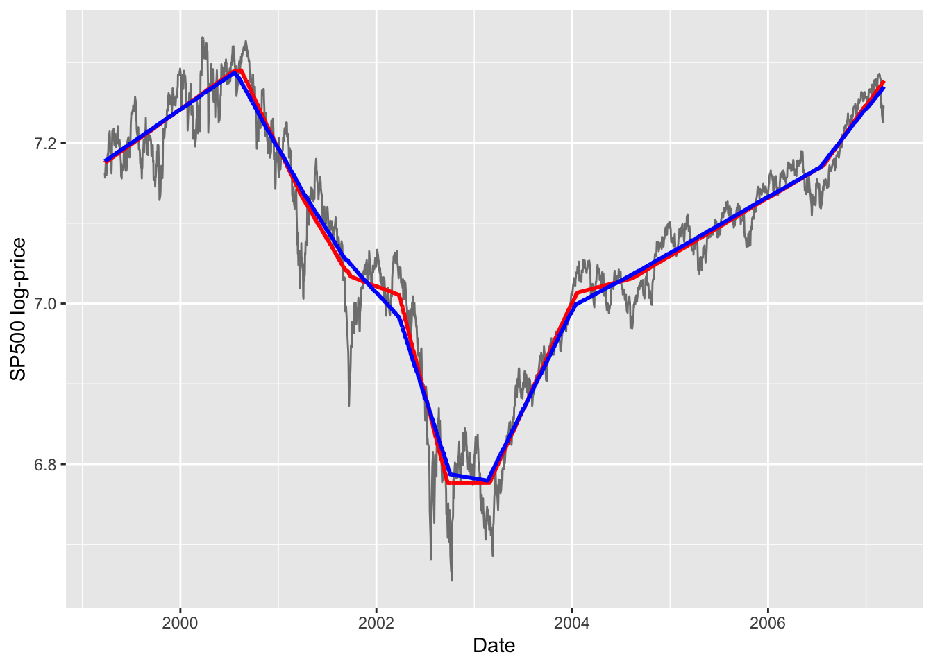
Next the corresponding CVXR plots.
cvxr_data <- data.frame(x = sp500$date,
                        y = sp500$log,
                        l1_50 = betaHat_50,
                        l1_100 = betaHat_100)
ggplot(data = cvxr_data) +
    geom_line(mapping = aes(x = x, y = y), color = 'grey50') +
    labs(x = "Date", y = "SP500 log-price") +
    geom_line(mapping = aes(x = x, y = l1_50), color = 'red', linewidth = 1) +
    geom_line(mapping = aes(x = x, y = l1_100), color = 'blue', linewidth = 1)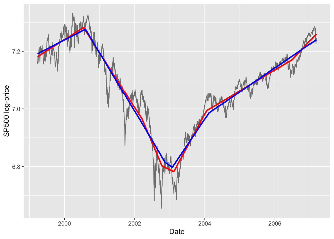
CVXR estimated \(L_1\) trends for \(\lambda = 50\) (red) and \(\lambda = 100\) (blue).Notes
The CVXR solution is not quite exactly that of l1tf: on the left it shows a larger difference for the two \(\lambda\) values; in the middle, it is less flatter than l1tf; and on the right, it does not have as many knots as l1tf.
Session Info
R version 4.6.0 (2026-04-24)
Platform: aarch64-apple-darwin23
Running under: macOS Tahoe 26.5.1

Matrix products: default
BLAS:   /Library/Frameworks/R.framework/Versions/4.6/Resources/lib/libRblas.0.dylib
LAPACK: /Library/Frameworks/R.framework/Versions/4.6/Resources/lib/libRlapack.dylib;  LAPACK version 3.12.1

locale:
[1] en_US.UTF-8/en_US.UTF-8/en_US.UTF-8/C/en_US.UTF-8/en_US.UTF-8

time zone: America/Los_Angeles
tzcode source: internal

attached base packages:
[1] stats     graphics  grDevices utils     datasets  methods   base

other attached packages:
[1] l1tf_0.0.0.9000 ggplot2_4.0.3   CVXR_1.9.1

loaded via a namespace (and not attached):
 [1] piqp_0.6.2         Matrix_1.7-5       gtable_0.3.6       jsonlite_2.0.0
 [5] dplyr_1.2.1        compiler_4.6.0     highs_1.14.0-2     tidyselect_1.2.1
 [9] Rcpp_1.1.1-1.1     slam_0.1-55        cccp_0.3-3         dichromat_2.0-0.1
[13] scales_1.4.0       yaml_2.3.12        fastmap_1.2.0      clarabel_0.11.2
[17] here_1.0.2         lattice_0.22-9     R6_2.6.1           labeling_0.4.3
[21] generics_0.1.4     knitr_1.51         htmlwidgets_1.6.4  backports_1.5.1
[25] checkmate_2.3.4    tibble_3.3.1       rprojroot_2.1.1    osqp_1.0.0
[29] pillar_1.11.1      RColorBrewer_1.1-3 rlang_1.2.0        xfun_0.58
[33] S7_0.2.2           otel_0.2.0         cli_3.6.6          withr_3.0.2
[37] magrittr_2.0.5     Rglpk_0.6-5.1      digest_0.6.39      grid_4.6.0
[41] gmp_0.7-5.1        lifecycle_1.0.5    ECOSolveR_0.6.1    scs_3.2.7
[45] vctrs_0.7.3        evaluate_1.0.5     glue_1.8.1         farver_2.1.2
[49] codetools_0.2-20   rmarkdown_2.31     pkgconfig_2.0.3    tools_4.6.0
[53] htmltools_0.5.9
References
Kim, Seung-Jean, Kwangmoo Koh, Stephen Boyd, and Dimitry Gorinevsky. 2009. “\(l_1\) Trend Filtering.” SIAM Review 51 (2): 339–60. https://doi.org/doi:10.1137/070690274.