## discrete-hazard counts for one (T, N) group
grp_counts <- function(T, N) {
  s  <- subset(oropharynx, tstage == T & nstage == N)
  dt <- sort(unique(s$days[s$status == 1]))            # distinct failure times
  out <- data.frame(t = dt,
             d = sapply(dt, function(x) sum(s$days == x & s$status == 1)),  # failures
             n = sapply(dt, function(x) sum(s$days >= x)))                  # at risk
  attr(out, "tmax") <- max(s$days)   # last observation, for the flat Kaplan-Meier tail
  out
}Stochastically Ordered Survival Functions
Introduction
In Estimating Stochastically Ordered Survival Functions via Geometric Programming, Lim et al. give a nice application of geometric programming to nonparametric estimation.
Suppose we have survival functions \(S_1, \ldots, S_N\) for \(N\) populations and prior knowledge that they are stochastically ordered. Two forms are common (Lim et al. 2009):
- Simple ordering, written \(S_a \preceq S_b\): population \(a\) dies stochastically earlier, i.e. \(S_a(t) \le S_b(t)\) for every \(t\).
- Uniform ordering: the ratio \(S_a(t)/S_b(t)\) is monotone in \(t\) — a stronger requirement that compares the two populations conditionally on survival so far, equivalent to an ordering of the hazard rates (Dykstra et al. 1991).
The unconstrained nonparametric maximum-likelihood estimates (NPMLEs) — Kaplan–Meier curves and their interval-censored analogues — often violate an ordering we believe on scientific grounds, crossing where they should not. Lim et al. (2009) observed that imposing the ordering turns the NPMLE into a geometric program (GP), and hence, in modern terms, a disciplined geometric program (DGP) (Agrawal et al. 2019) that CVXR can solve directly via psolve(prob, gp = TRUE).
We take up the easily-understood right-censored case first (Section 3 of the paper), then the interval-censored case (Section 4).
Geometric programs in one paragraph
A monomial is a function \(c\,x_1^{a_1}\cdots x_n^{a_n}\) with \(c > 0\), real exponents \(a_i\), and positive variables \(x_i\); a sum of monomials is a posynomial. A geometric program minimizes a posynomial subject to constraints of the form (posynomial \(\le 1\)) and (monomial \(= 1\)). The logarithmic change of variables \(x_i = e^{y_i}\) makes every such problem convex. CVXR recognizes this structure automatically: positive variables are declared with pos = TRUE, the objective and each constraint carry a log-log curvature, and is_dgp() checks that they compose into a valid program.
Right censoring
With right-censored data each subject either fails at an observed time or is known only to survive past its censoring time. Consider \(N\) populations. For population \(i\), let \(t_{i1} < \cdots < t_{i m_i}\) be its distinct observed failure times, and at \(t_{ij}\) let \[ n_{ij} = \#\{\text{subjects of population } i \text{ at risk just before } t_{ij}\}, \qquad d_{ij} = \#\{\text{failures at } t_{ij}\}. \]
The likelihood is a monomial
Define the discrete conditional survival probability \[ p_{ij} = P(Y_i > t_{ij} \mid Y_i > t_{i,j-1}) = \frac{S_i(t_{ij})}{S_i(t_{i,j-1})}, \qquad q_{ij} = 1 - p_{ij}, \] so that the survival function is the running product (the Kaplan–Meier form) \[ S_i(t_{ij}) = \prod_{r=1}^{j} p_{ir}. \] Conditionally on the \(n_{ij}\) subjects at risk, the \(d_{ij}\) failures are independent Bernoulli events: each subject fails at this instant with probability \(q_{ij}\) and survives it with probability \(p_{ij}\). So the \(t_{ij}\) term contributes \(q_{ij}^{d_{ij}} p_{ij}^{n_{ij} - d_{ij}}\), and the full likelihood is the monomial \[ \mathcal L = \prod_{i=1}^{N} \prod_{j=1}^{m_i} p_{ij}^{\,n_{ij} - d_{ij}}\, q_{ij}^{\,d_{ij}} . \] Because a monomial is log-log affine, the objective fits directly into a GP; the modeling work is in the constraints: that the \(p_{ij}, q_{ij}\) are probabilities, that survival is nonincreasing, and that the populations are ordered. As we will see, the sum-to-one constraint alone recovers the ordinary NPMLE (Kaplan–Meier), and the ordering monomials add the stochastic ordering.
Constraints
Sum-to-one (relaxed). Since \(p_{ij}\) and \(q_{ij}\) are complementary probabilities, \(p_{ij} + q_{ij} = 1\). A GP admits only monomial equalities, and \(p_{ij} + q_{ij}\) is a posynomial, so we relax to the posynomial inequality \[ p_{ij} + q_{ij} \le 1 . \] This is exact at the optimum: both exponents \(n_{ij} - d_{ij}\) and \(d_{ij}\) are nonnegative, so \(\mathcal L\) increases in each \(p_{ij}\) and \(q_{ij}\); wherever a variable is informative the optimizer pushes it up until the constraint binds.
Monotonicity is automatic. A survival curve must be nonincreasing. Here that is free: \(S_i(t_{ij}) = \prod_{r \le j} p_{ir}\) is a product of factors \(p_{ir} \le 1\), so it decreases in \(j\) with no extra constraint. (This is a genuine convenience of the conditional parameterization; the interval-censored model below is not so lucky.)
Simple ordering. “\(S_a\) stochastically smaller than \(S_b\)” means \(S_a(t) \le S_b(t)\) at every \(t\). Both survival curves are step functions that only change at failure times, so it suffices to enforce the inequality at each pooled failure time \(t\): \[ \prod_{r \,:\, t_{ar} \le t} p_{ar} \;\le\; \prod_{r \,:\, t_{br} \le t} p_{br} \quad\Longleftrightarrow\quad \Bigl(\textstyle\prod_{t_{ar} \le t} p_{ar}\Bigr) \Bigl(\textstyle\prod_{t_{br} \le t} p_{br}\Bigr)^{-1} \le 1, \] a monomial \(\le 1\). (Uniform ordering, when the two populations share a grid, is even simpler: \(p_{aj}\, p_{bj}^{-1} \le 1\) at each \(j\) — an ordering of the one-step conditional survival probabilities, i.e. of the discrete hazards.)
Everything is a monomial except \(p_{ij} + q_{ij} \le 1\) (a posynomial \(\le 1\)), so the problem is a DGP.
The oropharynx data
We use the oropharyngeal-carcinoma trial of Kalbfleisch and Prentice (192 patients, bundled with this example as oropharynx.rds). Following Lim et al. (2009) we group patients by tumor stage tstage (T) and nodal stage nstage (N), and model time to death.
CVXR implementation
fit_rc() builds the monomial likelihood, the relaxed sum-to-one constraints, and one simple-ordering monomial per pooled failure time for each requested pair. A pair c(a, b) requests \(S_a \le S_b\).
fit_rc <- function(groups, order = list()) {
  G <- length(groups)
  p <- lapply(groups, function(g) Variable(nrow(g), pos = TRUE))
  q <- lapply(groups, function(g) Variable(nrow(g), pos = TRUE))
  mono <- function(v, a) Reduce(`*`, lapply(which(a != 0), function(j) v[j]^a[j]))
  Scum <- function(i, ix) if (length(ix)) prod_entries(p[[i]][ix]) else 1   # empty prod = 1

  objective <- Reduce(`*`, lapply(seq_len(G), function(i)
                 mono(p[[i]], groups[[i]]$n - groups[[i]]$d) * mono(q[[i]], groups[[i]]$d)))
  constraints <- lapply(seq_len(G), function(i) p[[i]] + q[[i]] <= 1)

  for (o in order) {                     # S_a(t) <= S_b(t) at every pooled failure time
    a <- o[1]; b <- o[2]
    for (tk in sort(unique(c(groups[[a]]$t, groups[[b]]$t)))) {
      ia <- which(groups[[a]]$t <= tk); ib <- which(groups[[b]]$t <= tk)
      constraints <- c(constraints, Scum(a, ia) * Scum(b, ib)^(-1) <= 1)
    }
  }
  prob <- Problem(Maximize(objective), constraints)
  val  <- psolve(prob, gp = TRUE)
  check_solver_status(prob)
  list(is_dgp = is_dgp(prob), logLik = log(val),
       S = lapply(seq_len(G), function(i) cumprod(value(p[[i]]))))   # S = running product
}
A quick sanity check: with no ordering, the GP must return the ordinary Kaplan–Meier estimator.
g <- grp_counts(3, 3)
fit <- fit_rc(list(g))
km  <- survfit(Surv(days, status) ~ 1, data = subset(oropharynx, tstage == 3 & nstage == 3))
max(abs(fit$S[[1]] - summary(km, times = g$t)$surv))     # ~ 0: GP == Kaplan-Meier
[1] 1.796205e-05Simple ordering (paper Figure 1)
The paper’s first example takes the three T = 3 groups differing in nodal involvement, \((T,N) = (3,1), (3,2), (3,3)\), and imposes \(S_3 \preceq S_2 \preceq S_1\) (more nodal involvement, worse survival).
g1 <- list("(3,1)" = grp_counts(3, 1),
           "(3,2)" = grp_counts(3, 2),
           "(3,3)" = grp_counts(3, 3))

rc_free  <- fit_rc(g1)
rc_order <- fit_rc(g1, list(c(3, 2), c(2, 1)))     # S3 <= S2 <= S1

step_rc <- function(fit, groups, panel)
  do.call(rbind, lapply(seq_along(groups), function(i) {
    g <- groups[[i]]; S <- fit$S[[i]]; tmax <- attr(g, "tmax")
    t <- c(0, g$t); s <- c(1, S)
    if (tmax > max(g$t)) { t <- c(t, tmax); s <- c(s, tail(S, 1)) }  # flat KM tail to last obs
    data.frame(t = t, S = s, grp = paste0("(T,N)=", names(groups)[i]), panel = panel)
  }))

df1 <- rbind(step_rc(rc_free,  g1, "(a) Kaplan-Meier (unconstrained)"),
             step_rc(rc_order, g1, "(b) ordered: S3 <= S2 <= S1"))

ggplot(df1, aes(t, S, colour = grp)) + geom_step(linewidth = 0.6) +
  facet_wrap(~panel) + coord_cartesian(xlim = c(0, 1850), ylim = c(0, 1)) +
  labs(x = "time (days)", y = "survival probability", colour = NULL) +
  theme(legend.position = "inside", legend.position.inside = c(0.9, 0.8),
        legend.background = element_blank())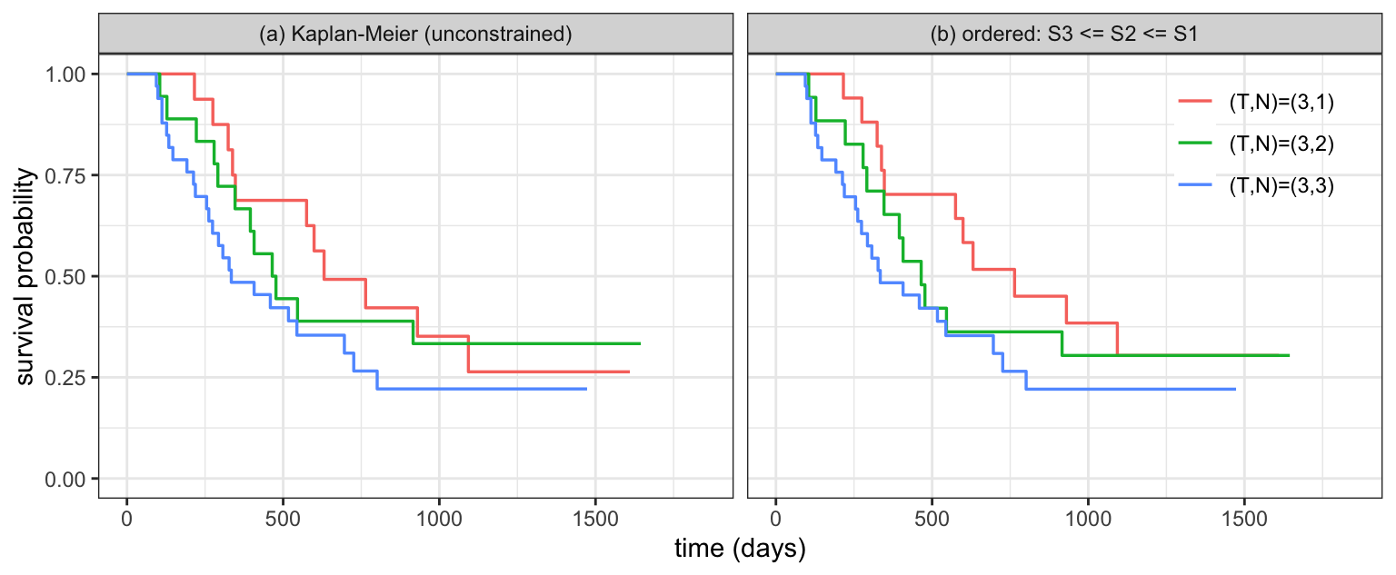
The unconstrained Kaplan–Meier curves cross — \((3,2)\) sits above \((3,1)\) for much of the range, contradicting \(S_2 \le S_1\). Imposing the ordering removes the crossings, reproducing Figure 1 of Lim et al. (2009).
c(unconstrained = round(rc_free$logLik, 2), ordered = round(rc_order$logLik, 2))unconstrained ordered
-169.15 -169.24 Partial ordering (paper Figure 2)
Ordering need not be a total order. For the four groups \((3,0), (3,3), (4,0), (4,3)\) — populations \(1\)–\(4\) — larger T or larger N should worsen survival, giving the partial order \(S_4 \preceq S_2 \preceq S_1\) and \(S_4 \preceq S_3 \preceq S_1\), while \(S_2\) and \(S_3\) are left incomparable. Each “\(\preceq\)” is just another list of pairs.
g2 <- list("(3,0)" = grp_counts(3, 0), "(3,3)" = grp_counts(3, 3),
           "(4,0)" = grp_counts(4, 0), "(4,3)" = grp_counts(4, 3))

pf_free  <- fit_rc(g2)
pf_order <- fit_rc(g2, list(c(4, 2), c(2, 1), c(4, 3), c(3, 1)))
Warning: Solution may be inaccurate. Try another solver, adjusting the solver settings,
or solve with `verbose = TRUE` for more information.df2 <- rbind(step_rc(pf_free, g2, "(a) Kaplan-Meier (unconstrained)"),
step_rc(pf_order, g2, "(b) partial order"))
ggplot(df2, aes(t, S, colour = grp)) + geom_step(linewidth = 0.6) +
facet_wrap(~panel) + coord_cartesian(xlim = c(0, 1850), ylim = c(0, 1)) +
labs(x = "time (days)", y = "survival probability", colour = NULL) +
theme(legend.position = "inside", legend.position.inside = c(0.9, 0.75),
legend.background = element_blank())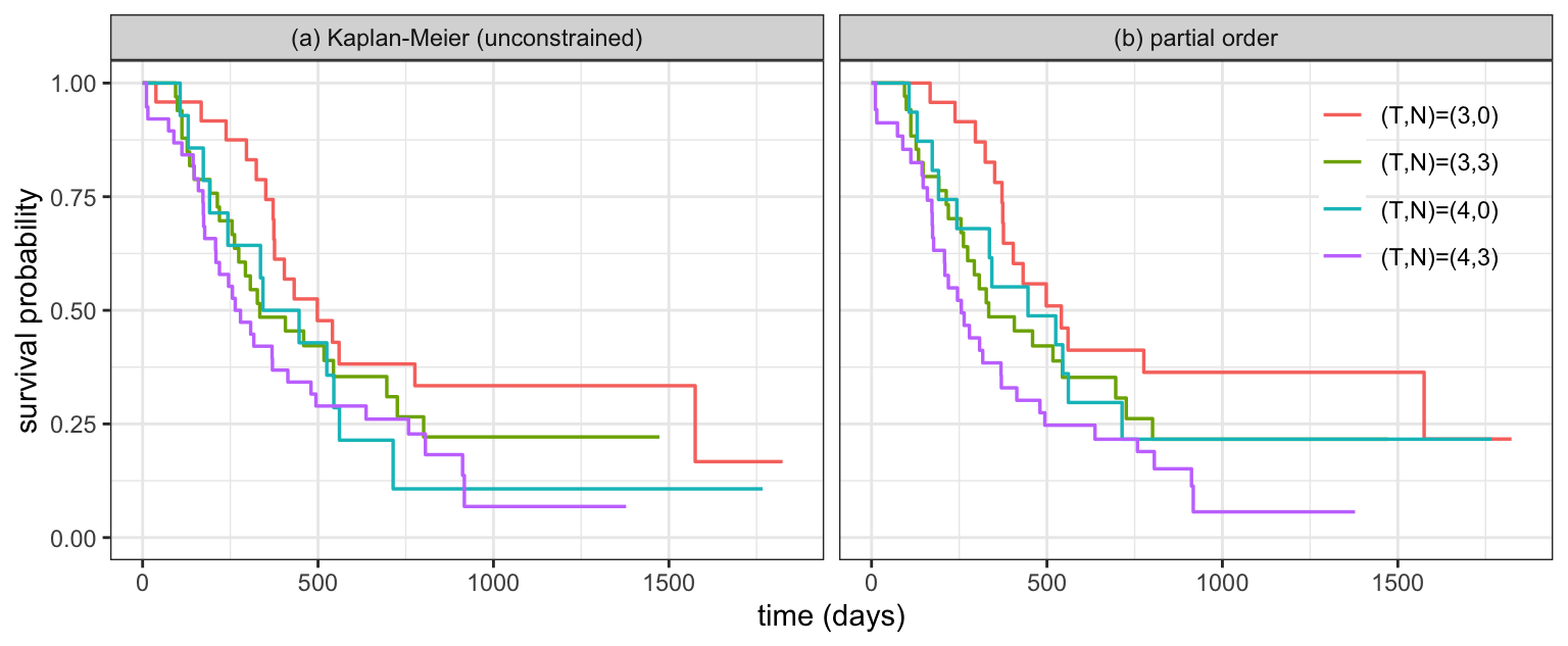
c(unconstrained = round(pf_free$logLik, 2), partial_order = round(pf_order$logLik, 2))unconstrained partial_order
-306.93 -327.88 Interval censoring
Right-censored data tell us a failure time exactly or bounds it below. Interval-censored data only bound it: the failure is known to lie between two examination times. The simplest form is “case 1” interval censoring, also called current-status data: each subject is examined exactly once, at a time \(C\), and all we learn is the single bit \(\delta = \mathbf 1\{Y \le C\}\) — whether the event has already happened. The failure time is thus known only to lie in \((0, C]\) (if \(\delta = 1\)) or in \((C, \infty)\) (if \(\delta = 0\)). (“Case 2” data have two examinations per subject and “case \(k\)” data have \(k\); see Sun (2006).) We treat case 1, as in Section 4.2 of Lim et al. (2009).
The likelihood is again a monomial
Consider \(N\) populations, pool all examination times into a common grid \(t_1 < \cdots < t_m\), and for population \(i\) at \(t_j\) let \[ n_{ij} = \#\{\text{subjects of population } i \text{ examined at } t_j\}, \qquad r_{ij} = \#\{\text{those with the event already present}\}. \] Because a subject examined at \(t_j\) has the event already present with probability \(P(Y_i \le t_j) = 1 - S_i(t_j)\), and these are independent, \(r_{ij} \sim \mathrm{Binomial}(n_{ij}, 1 - S_i(t_j))\). This time we parameterize directly with the survival values, \[ q_{ij} = S_i(t_j) \in (0, 1], \qquad p_{ij} = 1 - S_i(t_j), \] and the likelihood is the monomial \[ \mathcal L = \prod_{i=1}^{N} \prod_{j=1}^{m} p_{ij}^{\,r_{ij}}\, q_{ij}^{\,n_{ij} - r_{ij}} . \]
Constraints
Sum-to-one (relaxed) as before: \(p_{ij} + q_{ij} \le 1\), tight at the optimum for the same nonnegative-exponent reason.
Monotonicity is now explicit. Survival must be nonincreasing. Following the authors’ code we impose this on \(p_{ij} = 1 - S_i(t_j)\), making it nondecreasing, and read survival back as \(S_i(t_j) = 1 - p_{ij}\): \[ S_i(t_j) \ge S_i(t_{j+1}) \quad\Longleftrightarrow\quad p_{ij}\, p_{i,j+1}^{-1} \le 1, \] a monomial \(\le 1\) for \(j = 1, \ldots, m - 1\). This choice matters for the free early points. A population with no examinations yet has \(p_{ij}\) unconstrained by the data; because \(p\) increases from near 0, those values sit at ~0, so \(S = 1 - p\) stays at \(1\) until the first event — the standard survival convention, and exactly what the paper’s code produces with no ad-hoc adjustment. (Imposing monotonicity on \(q = S\) instead and reading \(S = q\) is algebraically equivalent but leaves those same free points centered below 1.)
Ordering. Both populations share the grid \(t_1, \ldots, t_m\).
- Simple, \(S_a \preceq S_b\) (population \(a\) smaller): \(1 - p_{aj} \le 1 - p_{bj} \Leftrightarrow p_{aj} \ge p_{bj}\), i.e. the monomial \(p_{bj}\, p_{aj}^{-1} \le 1\) at each \(t_j\).
- Uniform, “\(S_a\) uniformly larger than \(S_b\)”: the ratio \(S_a(t)/S_b(t)\) is nondecreasing, i.e. \(\dfrac{S_a(t_j)}{S_b(t_j)} \le \dfrac{S_a(t_{j+1})}{S_b(t_{j+1})}\). This is a monomial only in the survival variables \(q_{ij} = S_i(t_j)\); cross-multiplying (all terms positive), \[ q_{aj}\, q_{b,j+1} \le q_{a,j+1}\, q_{bj} \quad\Longleftrightarrow\quad q_{aj}\, q_{b,j+1}\, q_{a,j+1}^{-1}\, q_{bj}^{-1} \le 1. \]
So the simple-ordering fit works in \(p\) (survival \(1 - p\)), while uniform ordering works in the survival variables \(q\) directly. Uniform ordering implies simple ordering.
The lung-tumor data
The data are the germ-free-mouse experiment of Hoel and Walburg (1972), tabulated as Table 1.3 in Sun (2006). At death each mouse was autopsied for a lung tumor. Because the tumor is occult — present or not at death, and not the cause of death — each animal yields a single current-status observation: the death time is the examination time \(C\), and \(\delta = 1\) if a tumor was found. The two arms are
| Population | Environment | Mice | Found with tumor |
|---|---|---|---|
| 1 | conventional | 96 | 27 |
| 2 | germ-free | 47 | 35 |
(The two arms hold \(96 + 47 = 143\) animals in the data distributed with the paper; the study enrolled 144.) Pooling the death times gives \(m = 127\) distinct examination times (45–1008 days). The germ-free mice have the higher tumor prevalence, so their tumor-free survival sits below the conventional arm. Following Lim et al. (2009)’s Figure 4 we impose that germ-free tumor onset is stochastically earlier, \(S_2(t) \le S_1(t)\), which the unconstrained estimates violate at several times. (The text of §4.2 states the reverse, \(S_1 \le S_2\), but the paper’s supplementary code imposes \(S_2 \le S_1\) and its figure plots germ-free below — so we follow the code.)
CVXR implementation
Following the authors’ code, the builder parameterizes by \(p = 1 - S\) made monotone increasing, reads survival back as \(1 - p\), and takes the simple ordering as a function of the two p vectors.
monomial <- function(v, a) Reduce(`*`, lapply(which(a != 0), function(j) v[j]^a[j]))

fit_ic <- function(order_fun = function(p1, p2) list()) {
  p1 <- Variable(m, pos = TRUE); q1 <- Variable(m, pos = TRUE)  # population 1
  p2 <- Variable(m, pos = TRUE); q2 <- Variable(m, pos = TRUE)  # population 2

  objective <- monomial(p1, r1) * monomial(q1, n1 - r1) *
               monomial(p2, r2) * monomial(q2, n2 - r2)

  constraints <- c(
    list(p1 + q1 <= 1, p2 + q2 <= 1),                     # sum-to-one (relaxed)
    list(p1[1:(m-1)] <= p1[2:m], p2[1:(m-1)] <= p2[2:m]), # p increasing => S = 1-p decreasing
    order_fun(p1, p2))                                    # ordering monomials

  prob <- Problem(Maximize(objective), constraints)
  val  <- psolve(prob, gp = TRUE)
  check_solver_status(prob)
  list(is_dgp = is_dgp(prob), logLik = log(val), S1 = 1 - value(p1), S2 = 1 - value(p2))
}

no_order     <- function(p1, p2) list()
simple_order <- function(p1, p2) list(p1 <= p2)   # p1 <= p2  <=>  S1 >= S2 (germ-free below)
Simple ordering (paper Figure 4)
ic_free   <- fit_ic(no_order)
ic_simple <- fit_ic(simple_order)

step_ic <- function(fit, panel)
  rbind(data.frame(t = c(0, time), S = c(1, fit$S1), grp = "Conventional Env."),
        data.frame(t = c(0, time), S = c(1, fit$S2), grp = "Germ-free Env.")) |>
    transform(panel = panel)

df4 <- rbind(step_ic(ic_free,   "(a) not ordered"),
             step_ic(ic_simple, "(b) ordered: S2 <= S1"))

ggplot(df4, aes(t, S, colour = grp, linetype = grp)) +
  geom_step(linewidth = 0.5) + facet_wrap(~panel) +
  scale_colour_manual(values = c("Conventional Env." = "blue",
                                 "Germ-free Env." = "darkgreen")) +
  coord_cartesian(xlim = c(0, 1200), ylim = c(0, 1)) +
  labs(x = "time", y = "survival probability", colour = NULL, linetype = NULL) +
  theme(legend.position = "inside", legend.position.inside = c(0.79, 0.96),
        legend.justification.inside = c(0, 1), legend.background = element_blank())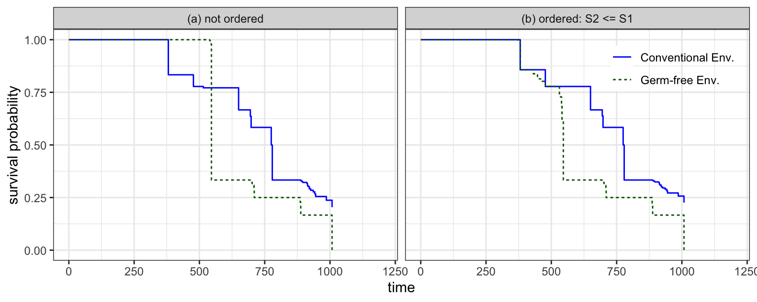
The unconstrained estimates keep conventional above germ-free but cross at several times where the germ-free curve pokes above. Imposing \(S_2 \le S_1\) removes those crossings — germ-free stays cleanly below conventional — reproducing Figure 4 of Lim et al. (2009). Both arms sit flat at \(1\) until their first tumor, as in the paper’s figure; this falls out of the \(p = 1-S\) parameterization with no plotting convention applied.
c(unconstrained_violations = sum(ic_free$S2   - ic_free$S1   > 1e-6),
  simple_violations        = sum(ic_simple$S2 - ic_simple$S1 > 1e-6))
unconstrained_violations simple_violations
22 0 Uniform ordering
Uniform ordering forces the ratio \(S_1/S_2\) to be monotone, so the curves may only diverge. Since it is a monomial only in the survival variables \(q\), this fit is built in \(q\) (made monotone decreasing) rather than in \(p\), and the survival is simply \(q\) itself. Imposed with conventional uniformly larger, it keeps conventional cleanly above germ-free with a widening gap; the uniform constraint pins the early free values, so the curves again sit flat at 1 before each first tumor.
fit_ic_uniform <- function() {
  p1 <- Variable(m, pos = TRUE); q1 <- Variable(m, pos = TRUE)
  p2 <- Variable(m, pos = TRUE); q2 <- Variable(m, pos = TRUE)
  objective <- monomial(p1, r1) * monomial(q1, n1 - r1) *
               monomial(p2, r2) * monomial(q2, n2 - r2)
  constraints <- c(
    list(p1 + q1 <= 1, p2 + q2 <= 1),
    list(q1[2:m] <= q1[1:(m-1)], q2[2:m] <= q2[1:(m-1)]),   # q monotone decreasing
    list(q1[1:(m-1)] * q2[2:m] <= q1[2:m] * q2[1:(m-1)]))   # S1/S2 nondecreasing
  prob <- Problem(Maximize(objective), constraints)
  val  <- psolve(prob, gp = TRUE); check_solver_status(prob)
  list(logLik = log(val), S1 = value(q1), S2 = value(q2))
}
ic_uniform <- fit_ic_uniform()

dfu <- rbind(step_ic(ic_free,    "x") |> transform(fit = "unconstrained"),
             step_ic(ic_uniform, "x") |> transform(fit = "uniform"))

ggplot(dfu, aes(t, S, colour = grp, linewidth = fit, alpha = fit)) +
  geom_step() +
  scale_colour_manual(values = c("Conventional Env." = "blue",
                                 "Germ-free Env." = "darkgreen")) +
  scale_linewidth_manual(values = c(unconstrained = 0.4, uniform = 1.0)) +
  scale_alpha_manual(values = c(unconstrained = 0.4, uniform = 1)) +
  coord_cartesian(xlim = c(0, 1200), ylim = c(0, 1)) +
  labs(x = "time", y = "survival probability",
       colour = NULL, linewidth = NULL, alpha = NULL) +
  theme(legend.position = "inside", legend.position.inside = c(0.72, 0.96),
        legend.justification.inside = c(0, 1), legend.background = element_blank())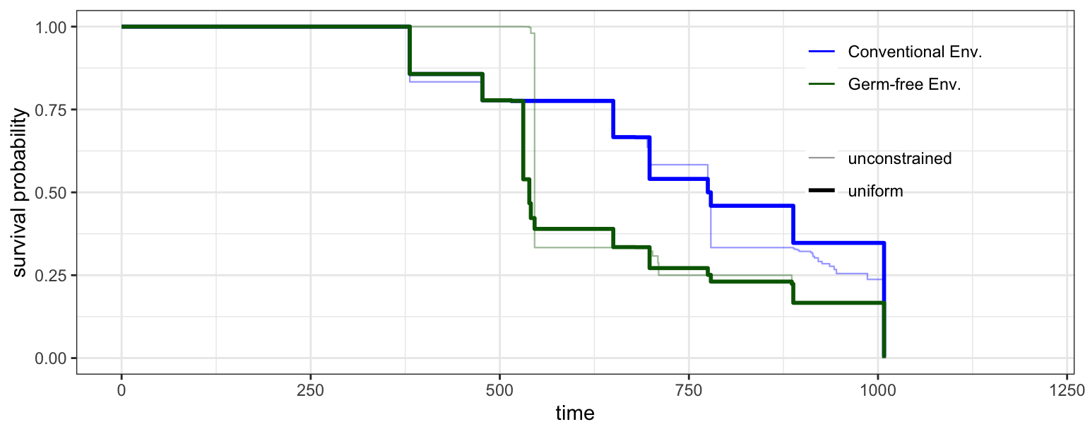
c(unconstrained_ratio_monotone = all(diff(ic_free$S1    / ic_free$S2)    >= -1e-6),
  uniform_ratio_monotone       = all(diff(ic_uniform$S1 / ic_uniform$S2) >= -1e-6))
unconstrained_ratio_monotone uniform_ratio_monotone
FALSE TRUE Notes
- The unconstrained NPMLE needs no GP at all:
survival::survfit()computes it directly — Kaplan–Meier for the right-censored groups, and the Turnbull (isotonic) estimator for the interval-censored case viaSurv(L, R, type = "interval2"). The GP with no ordering reproduces it (the Kaplan–Meier check above), so the GP earns its keep only for the ordering constraints, whichsurvfit()cannot impose; and the constrained log-likelihood is never above the unconstrained one. - The two censoring types use different parameterizations, and each gets a different constraint for free. The right-censored form uses the conditional survival \(p_{ij} = S_i(t_j)/S_i(t_{j-1})\) with \(S = \prod p\): monotonicity is automatic (each \(p \le 1\)), but simple ordering is a running-product inequality. The interval form uses \(p_{ij} = 1 - S_i(t_j)\) made monotone increasing with \(S = 1 - p\): monotonicity is an explicit constraint, but simple ordering is a single monomial at each time point (and uniform ordering a monomial in the survival variables \(q\)).
CVXR’spower()atom takes a scalar exponent, so a vector power such asq1^r1errors; the monomial is built as a product of scalar-power terms (themonomial()/mono()helpers).- At the optimum \(p + q = 1\) binds wherever the variable is informative. Where an exponent vanishes (e.g. an arm before its first examination) the survival value is not pinned by the data — a flat, non-unique stretch of the NPMLE. Which representative the solver returns depends on the parameterization: with \(p = 1-S\) monotone increasing those free values sit at ~0, so \(S = 1-p\) stays at 1 (the standard convention). This is a property of the parameterization, not a plotting fix-up — and it matches the paper’s supplementary code, which likewise reads \(S = 1 - p\).
Session Information
sessionInfo()R version 4.6.0 (2026-04-24)
Platform: aarch64-apple-darwin23
Running under: macOS Tahoe 26.5.1
Matrix products: default
BLAS: /Library/Frameworks/R.framework/Versions/4.6/Resources/lib/libRblas.0.dylib
LAPACK: /Library/Frameworks/R.framework/Versions/4.6/Resources/lib/libRlapack.dylib; LAPACK version 3.12.1
locale:
[1] en_US.UTF-8/en_US.UTF-8/en_US.UTF-8/C/en_US.UTF-8/en_US.UTF-8
time zone: America/Los_Angeles
tzcode source: internal
attached base packages:
[1] stats graphics grDevices utils datasets methods base
other attached packages:
[1] survival_3.8-6 ggplot2_4.0.3 CVXR_1.9.1
loaded via a namespace (and not attached):
[1] gmp_0.7-5.1 generics_0.1.4 clarabel_0.11.2 slam_0.1-55
[5] lattice_0.22-9 digest_0.6.39 magrittr_2.0.5 evaluate_1.0.5
[9] grid_4.6.0 RColorBrewer_1.1-3 fastmap_1.2.0 rprojroot_2.1.1
[13] jsonlite_2.0.0 Matrix_1.7-5 ECOSolveR_0.6.1 backports_1.5.1
[17] scs_3.2.7 scales_1.4.0 codetools_0.2-20 cli_3.6.6
[21] rlang_1.2.0 Rglpk_0.6-5.1 splines_4.6.0 withr_3.0.2
[25] yaml_2.3.12 otel_0.2.0 tools_4.6.0 osqp_1.0.0
[29] checkmate_2.3.4 dplyr_1.2.1 here_1.0.2 vctrs_0.7.3
[33] R6_2.6.1 lifecycle_1.0.5 htmlwidgets_1.6.4 pkgconfig_2.0.3
[37] cccp_0.3-3 pillar_1.11.1 gtable_0.3.6 glue_1.8.1
[41] Rcpp_1.1.1-1.1 xfun_0.58 tibble_3.3.1 tidyselect_1.2.1
[45] knitr_1.51 dichromat_2.0-0.1 highs_1.14.0-2 farver_2.1.2
[49] htmltools_0.5.9 rmarkdown_2.31 labeling_0.4.3 piqp_0.6.2
[53] compiler_4.6.0 S7_0.2.2 References
Agrawal, Akshay, Steven Diamond, and Stephen Boyd. 2019. “Disciplined Geometric Programming.” Optimization Letters 13 (5): 961–76. https://doi.org/10.1007/s11590-019-01422-z.
Dykstra, Richard, Subhash Kochar, and Tim Robertson. 1991. “Statistical Inference for Uniform Stochastic Ordering in Several Populations.” The Annals of Statistics 19 (2): 870–88.
Hoel, David G., and H. E. Walburg. 1972. “Statistical Analysis of Survival Experiments.” Journal of the National Cancer Institute 49 (2): 361–72.
Lim, Johan, Seung Jean Kim, and Xinlei Wang. 2009. “Estimating Stochastically Ordered Survival Functions via Geometric Programming.” Journal of Computational and Graphical Statistics 18 (4): 978–94. https://doi.org/10.1198/jcgs.2009.06140.
Sun, Jianguo. 2006. The Statistical Analysis of Interval-Censored Failure Time Data. Springer.