Lasso Regression

Author

CVXPY Developers and Balasubramanian Narasimhan

Introduction

Lasso regression is, like ridge regression, a shrinkage method. It differs from ridge regression in its choice of penalty: lasso imposes an $ℓ_{1}$ penalty on the parameters $β$ . That is, lasso finds an assignment to $β$ that minimizes the function

$f (β) = ∥ X β - Y ∥_{2}^{2} + λ ∥ β ∥_{1},$

where $λ$ is a hyperparameter and, as usual, $X$ is the training data and $Y$ the observations. The $ℓ_{1}$ penalty encourages sparsity in the learned parameters, and, as we will see, can drive many coefficients to zero. In this sense, lasso is a continuous feature selection method.

In this example, we show how to fit a lasso model using CVXR, how to evaluate the model, and how to tune the hyperparameter $λ$ .

Writing the Objective Function

We can decompose the objective function as the sum of a least squares loss function and an $ℓ_{1}$ regularizer.

In CVXR, we express the loss as sum_squares(X %*% beta - Y) (or equivalently p_norm(X %*% beta - Y, 2)^2) and the regularizer as p_norm(beta, 1). We also define a helper to compute the mean squared error (MSE) on any dataset.

loss_fn <- function(X, Y, beta) sum_squares(X %*% beta - Y)
regularizer <- function(beta) p_norm(beta, 1)
objective_fn <- function(X, Y, beta, lambd) {
    loss_fn(X, Y, beta) + lambd * regularizer(beta)
}
mse <- function(X, Y, beta) {
    (1.0 / nrow(X)) * value(loss_fn(X, Y, beta))
}

Generating Data

We generate training examples and observations that are linearly related; we make the relationship sparse, and we will see how lasso approximately recovers it.

set.seed(1)
m <- 100
n <- 20
sigma <- 5
density <- 0.2

## Generate sparse true coefficients
beta_star <- rnorm(n)
idxs <- sample.int(n, size = as.integer((1 - density) * n), replace = FALSE)
beta_star[idxs] <- 0

## Generate data matrix and observations
X <- matrix(rnorm(m * n), nrow = m, ncol = n)
Y <- X %*% beta_star + rnorm(m, sd = sigma)

## Split into train and test sets
X_train <- X[1:50, ]
Y_train <- Y[1:50]
X_test  <- X[51:100, ]
Y_test  <- Y[51:100]

Fitting the Model

All we need to do to fit the model is create a CVXR problem where the objective is to minimize the objective function defined above. We solve this for many values of $λ$ to obtain the regularization path.

beta <- Variable(n)

lambd_values <- 10^seq(-2, 3, length.out = 50)
train_errors <- numeric(length(lambd_values))
test_errors  <- numeric(length(lambd_values))
beta_values  <- vector("list", length(lambd_values))

for (i in seq_along(lambd_values)) {
    problem <- Problem(Minimize(objective_fn(X_train, Y_train, beta,
                                             lambd_values[i])))
    result <- psolve(problem)
    check_solver_status(problem)
    train_errors[i] <- mse(X_train, Y_train, beta)
    test_errors[i]  <- mse(X_test, Y_test, beta)
    beta_values[[i]] <- value(beta)
}

Evaluating the Model

Just as we saw for ridge regression, regularization improves generalizability. The plot below shows that, up to a point, increasing $λ$ reduces test error while increasing training error—the classic bias-variance trade-off.

df_error <- data.frame(lambda = lambd_values,
                       Train = train_errors,
                       Test = test_errors) |>
    pivot_longer(-lambda, names_to = "Set", values_to = "MSE")
ggplot(df_error, aes(x = lambda, y = MSE, color = Set)) +
    geom_line() +
    scale_x_log10() +
    scale_color_manual(values = c(Train = "blue", Test = "red")) +
    labs(x = expression(lambda), y = "Mean Squared Error (MSE)",
         title = "Mean Squared Error (MSE)") +
    theme_minimal()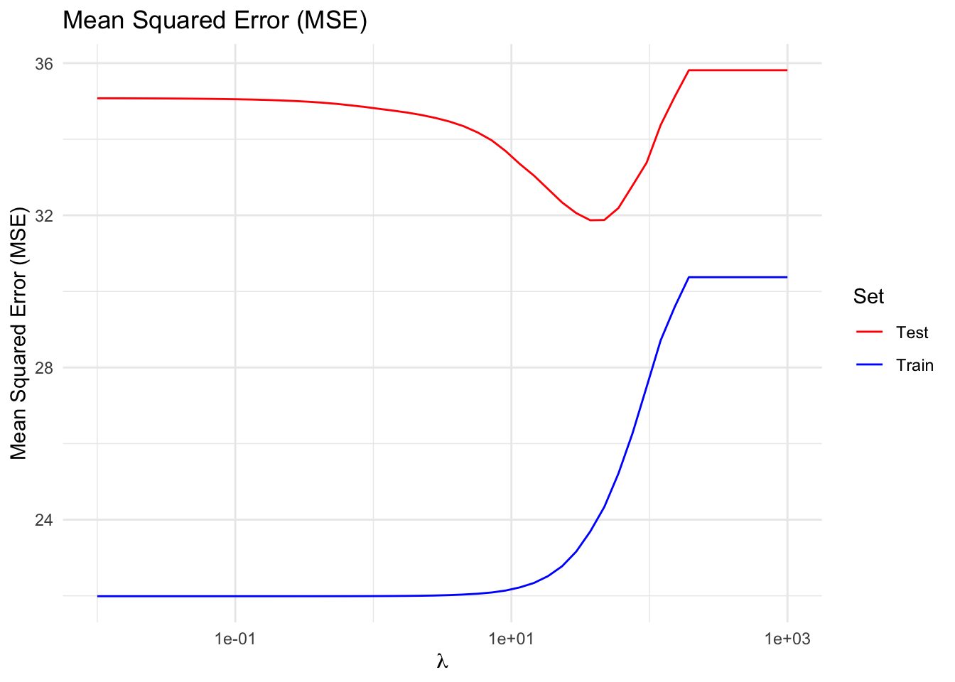

Regularization Path and Feature Selection

As $λ$ increases, the parameters are driven to $0$ . By $λ \approx 10$ , approximately 80 percent of the coefficients are exactly zero. This parallels the fact that $β^{*}$ was generated such that 80 percent of its entries were zero. The features corresponding to the slowest decaying coefficients can be interpreted as the most important ones.

Qualitatively, lasso differs from ridge in that the former often drives parameters to exactly zero, whereas the latter shrinks parameters but does not usually zero them out. That is, lasso results in sparse models; ridge (usually) does not.

beta_mat <- do.call(cbind, beta_values)
df_path <- data.frame(lambda = lambd_values, t(beta_mat)) |>
    pivot_longer(-lambda, names_to = "Coefficient", values_to = "Value")
ggplot(df_path, aes(x = lambda, y = Value, color = Coefficient)) +
    geom_line() +
    scale_x_log10() +
    labs(x = expression(lambda), y = expression(beta[i]),
         title = "Regularization Path") +
    theme_minimal() +
    guides(color = "none")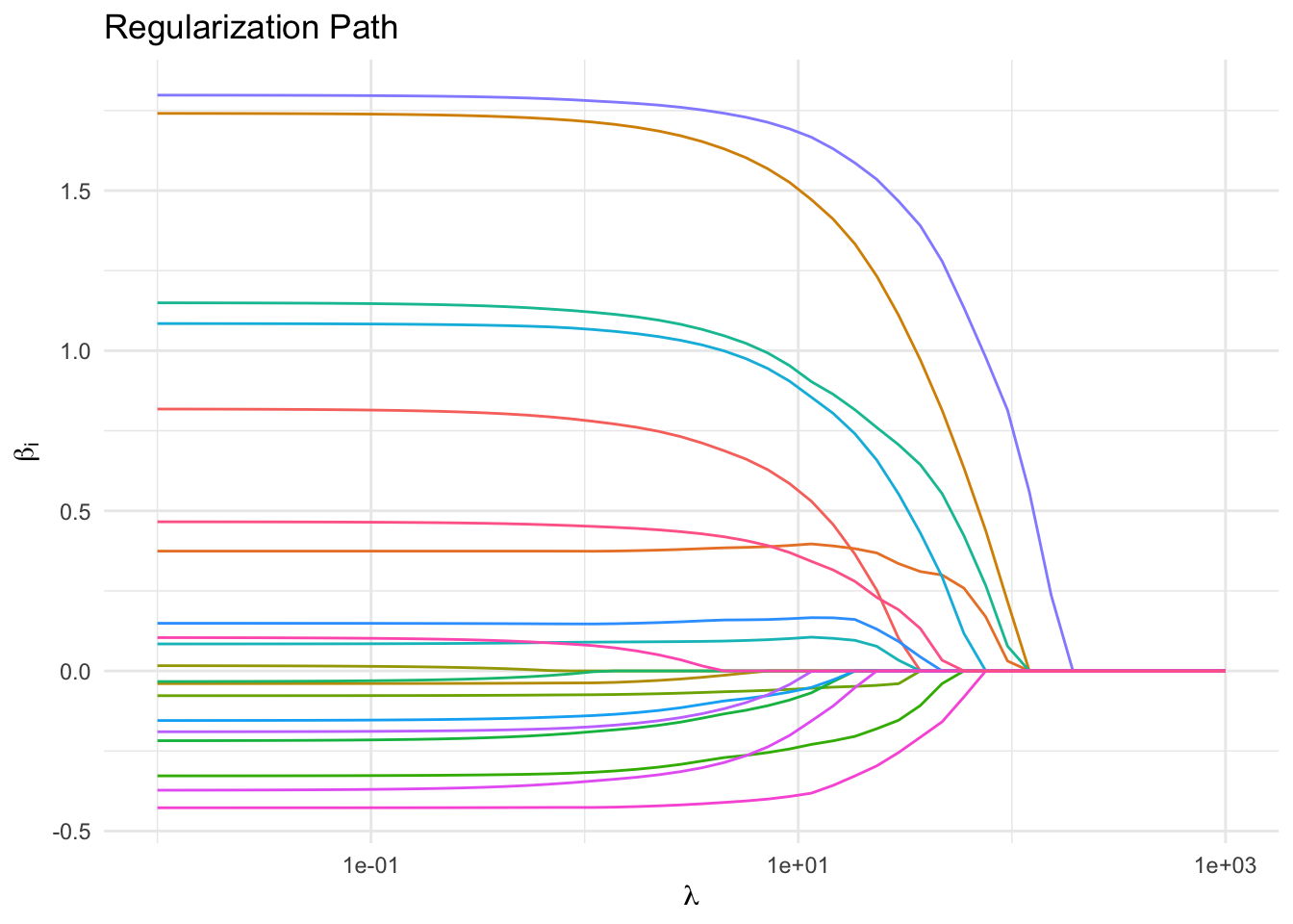

Session Info

R version 4.5.2 (2025-10-31)
Platform: aarch64-apple-darwin20
Running under: macOS Tahoe 26.3.1

Matrix products: default
BLAS:   /Library/Frameworks/R.framework/Versions/4.5-arm64/Resources/lib/libRblas.0.dylib 
LAPACK: /Library/Frameworks/R.framework/Versions/4.5-arm64/Resources/lib/libRlapack.dylib;  LAPACK version 3.12.1

locale:
[1] en_US.UTF-8/en_US.UTF-8/en_US.UTF-8/C/en_US.UTF-8/en_US.UTF-8

time zone: America/Los_Angeles
tzcode source: internal

attached base packages:
[1] stats     graphics  grDevices utils     datasets  methods   base     

other attached packages:
[1] tidyr_1.3.2   ggplot2_4.0.2 CVXR_1.8.1   

loaded via a namespace (and not attached):
 [1] gmp_0.7-5.1        generics_0.1.4     clarabel_0.11.2    slam_0.1-55       
 [5] lattice_0.22-9     digest_0.6.39      magrittr_2.0.4     evaluate_1.0.5    
 [9] grid_4.5.2         RColorBrewer_1.1-3 fastmap_1.2.0      rprojroot_2.1.1   
[13] jsonlite_2.0.0     Matrix_1.7-4       ECOSolveR_0.6.1    backports_1.5.0   
[17] scs_3.2.7          purrr_1.2.1        Rmosek_11.1.1      scales_1.4.0      
[21] codetools_0.2-20   cli_3.6.5          rlang_1.1.7        Rglpk_0.6-5.1     
[25] withr_3.0.2        yaml_2.3.12        otel_0.2.0         tools_4.5.2       
[29] osqp_1.0.0         Rcplex_0.3-8       checkmate_2.3.4    dplyr_1.2.0       
[33] here_1.0.2         gurobi_13.0-1      vctrs_0.7.1        R6_2.6.1          
[37] lifecycle_1.0.5    htmlwidgets_1.6.4  pkgconfig_2.0.3    cccp_0.3-3        
[41] pillar_1.11.1      gtable_0.3.6       glue_1.8.0         Rcpp_1.1.1        
[45] xfun_0.56          tibble_3.3.1       tidyselect_1.2.1   knitr_1.51        
[49] dichromat_2.0-0.1  highs_1.12.0-3     farver_2.1.2       htmltools_0.5.9   
[53] labeling_0.4.3     rmarkdown_2.30     piqp_0.6.2         compiler_4.5.2    
[57] S7_0.2.1