set.seed(1)
n <- 50
m <- 50

sigmoid <- function(z) 1 / (1 + exp(-z))

beta_true <- c(1, 0.5, -0.5, rep(0, n - 3))
X <- (matrix(runif(m * n), nrow = m, ncol = n) - 0.5) * 10
Y <- round(sigmoid(X %*% beta_true + rnorm(m, sd = 0.5)))

X_test <- (matrix(runif(2 * m * n), nrow = 2 * m, ncol = n) - 0.5) * 10
Y_test <- round(sigmoid(X_test %*% beta_true + rnorm(2 * m, sd = 0.5)))Logistic Regression with l1 Regularization
Introduction
In this example, we use CVXR to train a logistic regression classifier with \(\ell_1\) regularization. We are given data \((x_i, y_i)\), \(i = 1, \ldots, m\). The \(x_i \in \mathbf{R}^n\) are feature vectors, while the \(y_i \in \{0, 1\}\) are associated boolean classes.
Our goal is to construct a linear classifier \(\hat{y} = \mathbb{1}[\beta^T x > 0]\), which is \(1\) when \(\beta^T x\) is positive and \(0\) otherwise. We model the posterior probabilities of the classes given the data linearly, with
\[ \log \frac{\Pr(Y = 1 \mid X = x)}{\Pr(Y = 0 \mid X = x)} = \beta^T x. \]
This implies that
\[ \Pr(Y = 1 \mid X = x) = \frac{\exp(\beta^T x)}{1 + \exp(\beta^T x)}, \quad \Pr(Y = 0 \mid X = x) = \frac{1}{1 + \exp(\beta^T x)}. \]
We fit \(\beta\) by maximizing the log-likelihood of the data, plus a regularization term \(\lambda \|\beta\|_1\) with \(\lambda > 0\):
\[ \ell(\beta) = \sum_{i=1}^{m} y_i \beta^T x_i - \log(1 + \exp(\beta^T x_i)) - \lambda \|\beta\|_1. \]
Because \(\ell\) is a concave function of \(\beta\), this is a convex optimization problem.
Generating Data
In the following code we generate data with \(n = 50\) features by randomly choosing \(x_i\) and supplying a sparse \(\beta_{\text{true}} \in \mathbf{R}^n\). We then set \(y_i = \mathbb{1}[\beta_{\text{true}}^T x_i + z_i > 0]\), where the \(z_i\) are i.i.d. normal random variables. We divide the data into training and test sets with \(m = 50\) examples each.
Formulating the Problem
We next formulate the optimization problem using CVXR. The logistic atom in CVXR computes \(f(z) = \log(1 + e^z)\), which we use to express the log-likelihood.
beta <- Variable(n)
log_likelihood <- sum_entries(
    Y * (X %*% beta) - logistic(X %*% beta)
)
Fitting the Model
We solve the optimization problem for a range of \(\lambda\) to compute a trade-off curve. We then plot the train and test error over the trade-off curve. A reasonable choice of \(\lambda\) is the value that minimizes the test error.
## Classification error function
calc_error <- function(scores, labels) {
    preds <- ifelse(scores > 0, 1, 0)
    sum(abs(preds - labels)) / length(labels)
}
trials <- 100
train_error <- numeric(trials)
test_error <- numeric(trials)
lambda_vals <- 10^seq(-2, 0, length.out = trials)
beta_vals <- vector("list", trials)
for (i in seq_len(trials)) {
problem <- Problem(Maximize(log_likelihood / m -
lambda_vals[i] * p_norm(beta, 1)))
result <- psolve(problem)
check_solver_status(problem)
beta_hat <- value(beta)
train_error[i] <- calc_error(X %*% beta_hat, Y)
test_error[i] <- calc_error(X_test %*% beta_hat, Y_test)
beta_vals[[i]] <- beta_hat
}Warning: Solution may be inaccurate. Try another solver, adjusting the solver settings,
or solve with `verbose = TRUE` for more information.df_error <- data.frame(lambda = lambda_vals,
Train = train_error,
Test = test_error) |>
pivot_longer(-lambda, names_to = "Set", values_to = "Error")
ggplot(df_error, aes(x = lambda, y = Error, color = Set)) +
geom_line() +
scale_x_log10() +
scale_color_manual(values = c(Train = "blue", Test = "red")) +
labs(x = expression(lambda), y = "Classification Error",
title = "Train vs. Test Error") +
theme_minimal()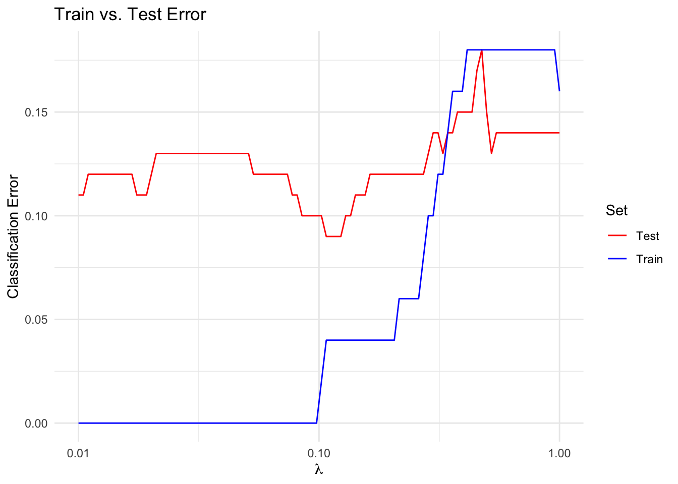
Regularization Path
We also plot the regularization path, or the \(\beta_i\) versus \(\lambda\). Notice that a few features remain non-zero longer for larger \(\lambda\) than the rest, which suggests that these features are the most important.
beta_mat <- do.call(cbind, beta_vals)
df_path <- data.frame(lambda = lambda_vals, t(beta_mat)) |>
    pivot_longer(-lambda, names_to = "Coefficient", values_to = "Value")
ggplot(df_path, aes(x = lambda, y = Value, color = Coefficient)) +
    geom_line() +
    scale_x_log10() +
    labs(x = expression(lambda), y = expression(beta[i]),
         title = "Regularization Path") +
    theme_minimal() +
    guides(color = "none")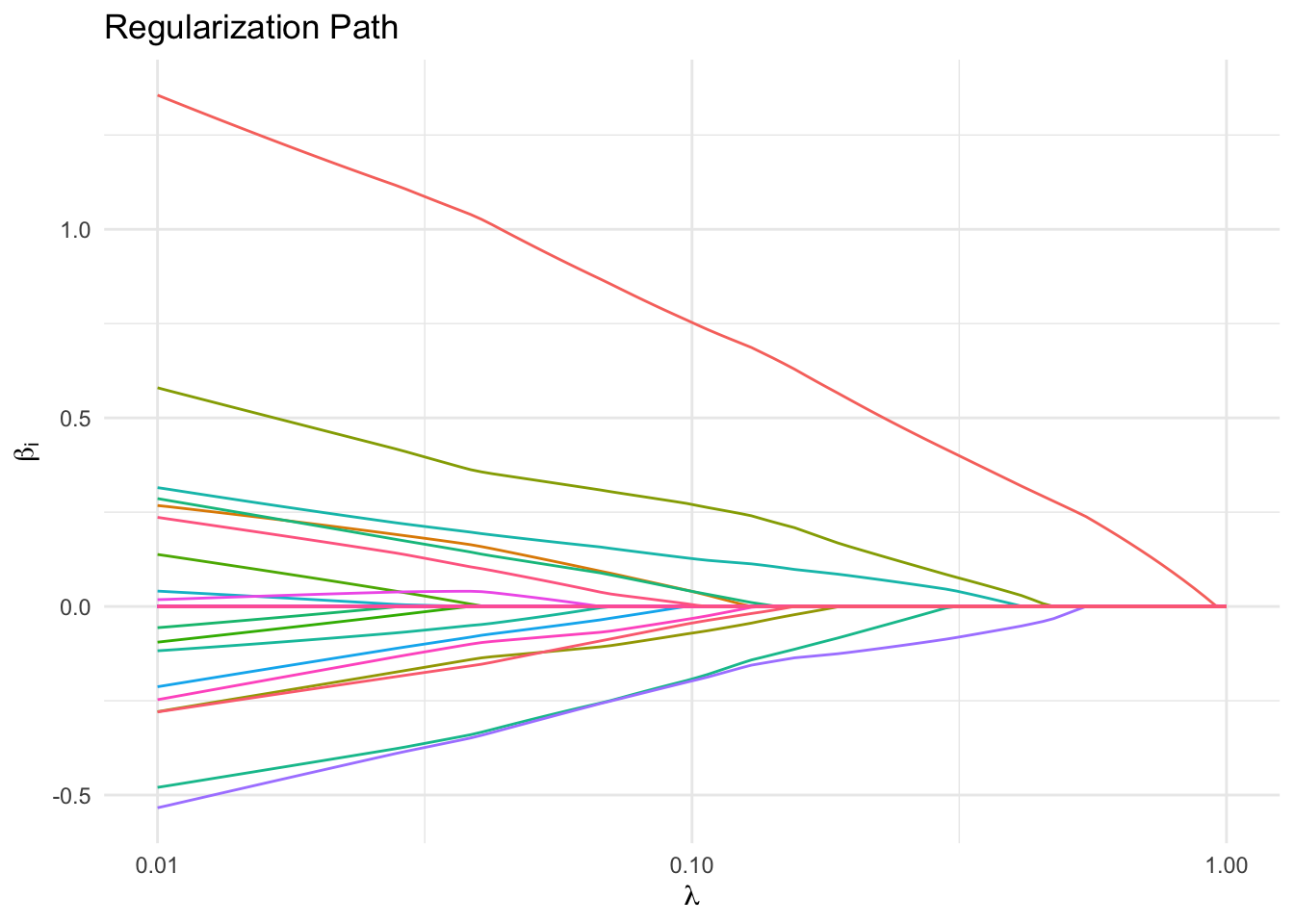
Comparing True and Reconstructed Coefficients
We plot the true \(\beta\) versus the reconstructed \(\beta\), as chosen to minimize error on the test set. The non-zero coefficients are reconstructed with good accuracy. There are a few values in the reconstructed \(\beta\) that are non-zero but should be zero.
idx <- which.min(test_error)
df_coef <- data.frame(i = seq_along(beta_true),
                      True = beta_true,
                      Reconstructed = drop(beta_vals[[idx]])) |>
    pivot_longer(-i, names_to = "Type", values_to = "Value")
ggplot(df_coef, aes(x = i, y = Value, color = Type)) +
    geom_line() +
    scale_color_manual(values = c(True = "blue", Reconstructed = "red")) +
    labs(x = "i", y = expression(beta[i]),
         title = "True vs. Reconstructed Coefficients") +
    theme_minimal()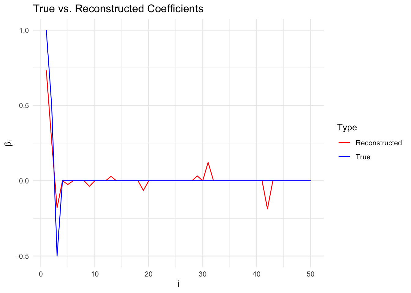
Session Info
R version 4.6.0 (2026-04-24)
Platform: aarch64-apple-darwin23
Running under: macOS Tahoe 26.5.1

Matrix products: default
BLAS:   /Library/Frameworks/R.framework/Versions/4.6/Resources/lib/libRblas.0.dylib
LAPACK: /Library/Frameworks/R.framework/Versions/4.6/Resources/lib/libRlapack.dylib;  LAPACK version 3.12.1

locale:
[1] en_US.UTF-8/en_US.UTF-8/en_US.UTF-8/C/en_US.UTF-8/en_US.UTF-8

time zone: America/Los_Angeles
tzcode source: internal

attached base packages:
[1] stats     graphics  grDevices utils     datasets  methods   base

other attached packages:
[1] tidyr_1.3.2   ggplot2_4.0.3 CVXR_1.9.1

loaded via a namespace (and not attached):
 [1] gmp_0.7-5.1        generics_0.1.4     clarabel_0.11.2    slam_0.1-55
 [5] lattice_0.22-9     digest_0.6.39      magrittr_2.0.5     evaluate_1.0.5
 [9] grid_4.6.0         RColorBrewer_1.1-3 fastmap_1.2.0      rprojroot_2.1.1
[13] jsonlite_2.0.0     Matrix_1.7-5       ECOSolveR_0.6.1    backports_1.5.1
[17] scs_3.2.7          purrr_1.2.2        scales_1.4.0       codetools_0.2-20
[21] cli_3.6.6          rlang_1.2.0        Rglpk_0.6-5.1      withr_3.0.2
[25] yaml_2.3.12        otel_0.2.0         tools_4.6.0        osqp_1.0.0
[29] checkmate_2.3.4    dplyr_1.2.1        here_1.0.2         vctrs_0.7.3
[33] R6_2.6.1           lifecycle_1.0.5    htmlwidgets_1.6.4  pkgconfig_2.0.3
[37] cccp_0.3-3         pillar_1.11.1      gtable_0.3.6       glue_1.8.1
[41] Rcpp_1.1.1-1.1     xfun_0.58          tibble_3.3.1       tidyselect_1.2.1
[45] knitr_1.51         dichromat_2.0-0.1  highs_1.14.0-2     farver_2.1.2
[49] htmltools_0.5.9    rmarkdown_2.31     labeling_0.4.3     piqp_0.6.2
[53] compiler_4.6.0     S7_0.2.2