Ridge Regression

Author

CVXPY Developers and Balasubramanian Narasimhan

Introduction

Ridge regression is a regression technique that is quite similar to unadorned least squares linear regression: simply adding an $ℓ_{2}$ penalty on the parameters $β$ to the objective function for linear regression yields the objective function for ridge regression.

Our goal is to find an assignment to $β$ that minimizes the function

$f (β) = ∥ X β - Y ∥_{2}^{2} + λ ∥ β ∥_{2}^{2},$

where $λ$ is a hyperparameter and, as usual, $X$ is the training data and $Y$ the observations. In practice, we tune $λ$ until we find a model that generalizes well to the test data.

Ridge regression is an example of a shrinkage method: compared to least squares, it shrinks the parameter estimates in the hopes of reducing variance, improving prediction accuracy, and aiding interpretation.

In this example, we show how to fit a ridge regression model using CVXR, how to evaluate the model, and how to tune the hyperparameter $λ$ .

Writing the Objective Function

We can decompose the objective function as the sum of a least squares loss function and an $ℓ_{2}$ regularizer.

loss_fn <- function(X, Y, beta) p_norm(X %*% beta - Y, 2)^2
regularizer <- function(beta) p_norm(beta, 2)^2
objective_fn <- function(X, Y, beta, lambd) {
    loss_fn(X, Y, beta) + lambd * regularizer(beta)
}
mse <- function(X, Y, beta) {
    (1.0 / nrow(X)) * value(loss_fn(X, Y, beta))
}

Generating Data

Because ridge regression encourages the parameter estimates to be small, it tends to lead to models with less variance than those fit with vanilla linear regression. We generate a small dataset that will illustrate this.

set.seed(1)
m <- 100
n <- 20
sigma <- 5

## Generate true coefficients
beta_star <- rnorm(n)

## Generate an ill-conditioned data matrix
X <- matrix(rnorm(m * n), nrow = m, ncol = n)

## Corrupt the observations with additive Gaussian noise
Y <- X %*% beta_star + rnorm(m, sd = sigma)

## Split into train and test sets
X_train <- X[1:50, ]
Y_train <- Y[1:50]
X_test  <- X[51:100, ]
Y_test  <- Y[51:100]

Fitting the Model

All we need to do to fit the model is create a CVXR problem where the objective is to minimize the objective function defined above. We solve this for many values of $λ$ to obtain the regularization path.

beta <- Variable(n)

lambd_values <- 10^seq(-2, 2, length.out = 50)
train_errors <- numeric(length(lambd_values))
test_errors  <- numeric(length(lambd_values))
beta_values  <- vector("list", length(lambd_values))

for (i in seq_along(lambd_values)) {
    problem <- Problem(Minimize(objective_fn(X_train, Y_train, beta,
                                             lambd_values[i])))
    result <- psolve(problem, solver = "CLARABEL")
    check_solver_status(problem)
    train_errors[i] <- mse(X_train, Y_train, beta)
    test_errors[i]  <- mse(X_test, Y_test, beta)
    beta_values[[i]] <- value(beta)
}

Warning: Solution may be inaccurate. Try another solver, adjusting the solver settings,
or solve with `verbose = TRUE` for more information.
Solution may be inaccurate. Try another solver, adjusting the solver settings,
or solve with `verbose = TRUE` for more information.
Solution may be inaccurate. Try another solver, adjusting the solver settings,
or solve with `verbose = TRUE` for more information.

Evaluating the Model

Notice that, up to a point, penalizing the size of the parameters reduces test error at the cost of increasing the training error, trading off higher bias for lower variance; in other words, this indicates that, for our example, a properly tuned ridge regression generalizes better than a least squares linear regression.

df_error <- data.frame(lambda = lambd_values,
                       Train = train_errors,
                       Test = test_errors) |>
    pivot_longer(-lambda, names_to = "Set", values_to = "MSE")
ggplot(df_error, aes(x = lambda, y = MSE, color = Set)) +
    geom_line() +
    scale_x_log10() +
    scale_color_manual(values = c(Train = "blue", Test = "red")) +
    labs(x = expression(lambda), y = "Mean Squared Error (MSE)",
         title = "Mean Squared Error (MSE)") +
    theme_minimal()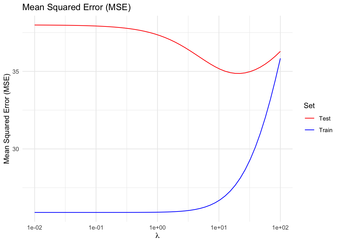

Regularization Path

As expected, increasing $λ$ drives the parameters towards $0$ . In a real-world example, those parameters that approach zero slower than others might correspond to the more informative features. It is in this sense that ridge regression can be considered model selection.

beta_mat <- do.call(cbind, beta_values)
df_path <- data.frame(lambda = lambd_values, t(beta_mat)) |>
    pivot_longer(-lambda, names_to = "Coefficient", values_to = "Value")
ggplot(df_path, aes(x = lambda, y = Value, color = Coefficient)) +
    geom_line() +
    scale_x_log10() +
    labs(x = expression(lambda), y = expression(beta[i]),
         title = "Regularization Path") +
    theme_minimal() +
    guides(color = "none")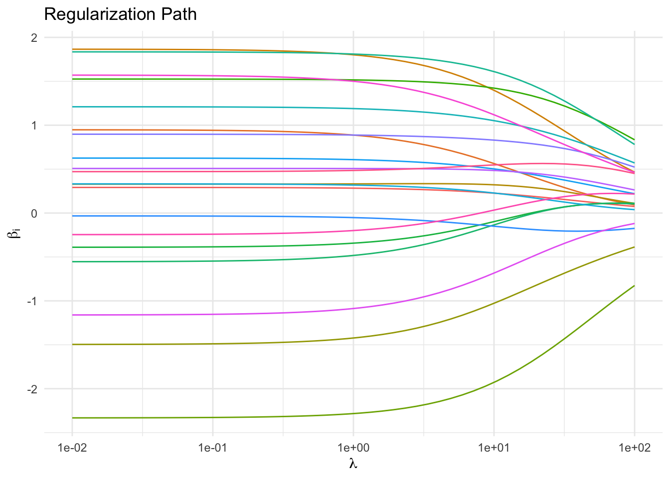

Session Info

R version 4.5.2 (2025-10-31)
Platform: aarch64-apple-darwin20
Running under: macOS Tahoe 26.3

Matrix products: default
BLAS:   /Library/Frameworks/R.framework/Versions/4.5-arm64/Resources/lib/libRblas.0.dylib 
LAPACK: /Library/Frameworks/R.framework/Versions/4.5-arm64/Resources/lib/libRlapack.dylib;  LAPACK version 3.12.1

locale:
[1] en_US.UTF-8/en_US.UTF-8/en_US.UTF-8/C/en_US.UTF-8/en_US.UTF-8

time zone: America/Los_Angeles
tzcode source: internal

attached base packages:
[1] stats     graphics  grDevices utils     datasets  methods   base     

other attached packages:
[1] tidyr_1.3.2   ggplot2_4.0.2 CVXR_1.8.1   

loaded via a namespace (and not attached):
 [1] gmp_0.7-5.1        generics_0.1.4     clarabel_0.11.2    slam_0.1-55       
 [5] lattice_0.22-9     digest_0.6.39      magrittr_2.0.4     evaluate_1.0.5    
 [9] grid_4.5.2         RColorBrewer_1.1-3 fastmap_1.2.0      rprojroot_2.1.1   
[13] jsonlite_2.0.0     Matrix_1.7-4       ECOSolveR_0.6.1    backports_1.5.0   
[17] scs_3.2.7          purrr_1.2.1        Rmosek_11.1.1      scales_1.4.0      
[21] codetools_0.2-20   cli_3.6.5          rlang_1.1.7        Rglpk_0.6-5.1     
[25] withr_3.0.2        yaml_2.3.12        otel_0.2.0         tools_4.5.2       
[29] osqp_1.0.0         Rcplex_0.3-8       checkmate_2.3.4    dplyr_1.2.0       
[33] here_1.0.2         gurobi_13.0-1      vctrs_0.7.1        R6_2.6.1          
[37] lifecycle_1.0.5    htmlwidgets_1.6.4  pkgconfig_2.0.3    cccp_0.3-3        
[41] pillar_1.11.1      gtable_0.3.6       glue_1.8.0         Rcpp_1.1.1        
[45] xfun_0.56          tibble_3.3.1       tidyselect_1.2.1   knitr_1.51        
[49] dichromat_2.0-0.1  highs_1.12.0-3     farver_2.1.2       htmltools_0.5.9   
[53] labeling_0.4.3     rmarkdown_2.30     piqp_0.6.2         compiler_4.5.2    
[57] S7_0.2.1