Quantile Regression

Author

Anqi Fu and Balasubramanian Narasimhan

Introduction

Quantile regression is another variation on least squares . The loss is the tilted $l_{1}$ function,

$ϕ (u) = τ max (u, 0) - (1 - τ) max (- u, 0) = \frac{1}{2} | u | + (τ - \frac{1}{2}) u,$

where $τ \in (0, 1)$ specifies the quantile. The problem as before is to minimize the total residual loss. This model is commonly used in ecology, healthcare, and other fields where the mean alone is not enough to capture complex relationships between variables. CVXR allows us to create a function to represent the loss and integrate it seamlessly into the problem definition, as illustrated below.

Example

We will use an example from the quantreg package. The vignette provides an example of the estimation and plot.

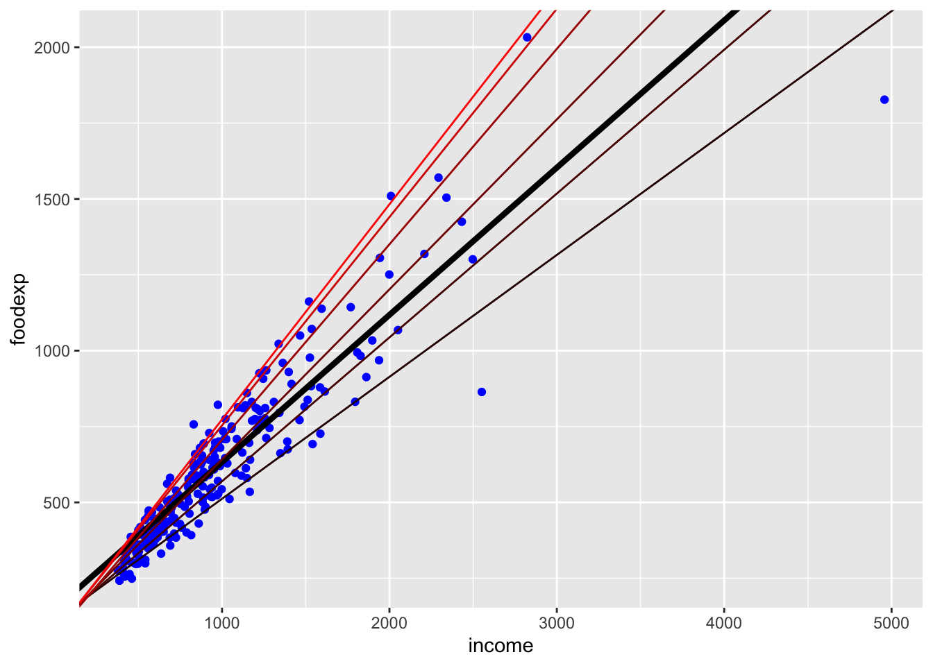
data(engel)
p <- ggplot(data = engel) +
    geom_point(mapping = aes(x = income, y = foodexp), color = "blue")
taus <- c(0.1, 0.25, 0.5, 0.75, 0.90, 0.95)
fits <- data.frame(
    coef(lm(foodexp ~ income, data = engel)),
    sapply(taus, function(x) coef(rq(formula = foodexp ~ income, data = engel, tau = x))))
names(fits) <- c("OLS", sprintf("\\(\\tau_{%0.2f}\\)", taus))

nf <- ncol(fits)
colors <- colorRampPalette(colors = c("black", "red"))(nf)
p <- p + geom_abline(intercept = fits[1, 1], slope = fits[2, 1], color = colors[1], linewidth = 1.5)
for (i in seq_len(nf)[-1]) {
    p <- p + geom_abline(intercept = fits[1, i], slope = fits[2, i], color = colors[i])
}
p

The above plot shows the quantile regression fits for $τ = (0.1, 0.25, 0.5, 0.75, 0.90, 0.95)$ . The OLS fit is the thick black line.

The following is a table of the estimates.

knitr::kable(fits, format = "html", escape = FALSE, caption = "Fits from OLS and `quantreg`") |>
    kable_styling("striped") |>
    column_spec(1:8, background = "#ececec")

Fits from OLS and `quantreg`
	OLS	$τ_{0.10}$	$τ_{0.25}$	$τ_{0.50}$	$τ_{0.75}$	$τ_{0.90}$	$τ_{0.95}$
(Intercept)	147.4753885	110.1415742	95.4835396	81.4822474	62.3965855	67.3508721	64.1039632
income	0.4851784	0.4017658	0.4741032	0.5601806	0.6440141	0.6862995	0.7090685

The CVXR formulation follows. Note we make use of model.matrix to get the intercept column painlessly.

X <- model.matrix(foodexp ~ income, data = engel)
y <- matrix(engel[, "foodexp"], ncol = 1)
beta <- Variable(2)
quant_loss <- function(u, tau) { 0.5 * abs(u) + (tau - 0.5) * u }
solutions <- sapply(taus, function(tau) {
    obj <- sum(quant_loss(y - X %*% beta, tau = tau))
    prob <- Problem(Minimize(obj))
    ## THE OSQP solver returns an error for tau = 0.5
    psolve(prob, solver = "CLARABEL")
    check_solver_status(prob)
    value(beta)
})
fits <- data.frame(coef(lm(foodexp ~ income, data = engel)),
                   solutions)
names(fits) <- c("OLS", sprintf("\\(\\tau_{%0.2f}\\)", taus))

Here is a table similar to the above with the OLS estimate added in for easy comparison.

knitr::kable(fits, format = "html", escape = FALSE, caption = "Fits from OLS and `CVXR`") |>
    kable_styling("striped") |>
    column_spec(1:8, background = "#ececec")

Fits from OLS and `CVXR`
	OLS	$τ_{0.10}$	$τ_{0.25}$	$τ_{0.50}$	$τ_{0.75}$	$τ_{0.90}$	$τ_{0.95}$
(Intercept)	147.4753885	110.1415744	95.4835346	81.4822479	62.3965859	67.3508715	64.1039637
income	0.4851784	0.4017658	0.4741032	0.5601806	0.6440141	0.6862995	0.7090685

The results match.

Session Info

R version 4.5.2 (2025-10-31)
Platform: aarch64-apple-darwin20
Running under: macOS Tahoe 26.3

Matrix products: default
BLAS:   /Library/Frameworks/R.framework/Versions/4.5-arm64/Resources/lib/libRblas.0.dylib 
LAPACK: /Library/Frameworks/R.framework/Versions/4.5-arm64/Resources/lib/libRlapack.dylib;  LAPACK version 3.12.1

locale:
[1] en_US.UTF-8/en_US.UTF-8/en_US.UTF-8/C/en_US.UTF-8/en_US.UTF-8

time zone: America/Los_Angeles
tzcode source: internal

attached base packages:
[1] stats     graphics  grDevices utils     datasets  methods   base     

other attached packages:
[1] quantreg_6.1     SparseM_1.84-2   kableExtra_1.4.0 ggplot2_4.0.2   
[5] CVXR_1.8.1      

loaded via a namespace (and not attached):
 [1] gtable_0.3.6       xfun_0.56          htmlwidgets_1.6.4  lattice_0.22-9    
 [5] vctrs_0.7.1        tools_4.5.2        Rmosek_11.1.1      generics_0.1.4    
 [9] tibble_3.3.1       highs_1.12.0-3     pkgconfig_2.0.3    piqp_0.6.2        
[13] Matrix_1.7-4       checkmate_2.3.4    RColorBrewer_1.1-3 S7_0.2.1          
[17] lifecycle_1.0.5    compiler_4.5.2     farver_2.1.2       stringr_1.6.0     
[21] MatrixModels_0.5-4 textshaping_1.0.4  gurobi_13.0-1      codetools_0.2-20  
[25] ECOSolveR_0.6.1    htmltools_0.5.9    cccp_0.3-3         yaml_2.3.12       
[29] gmp_0.7-5.1        pillar_1.11.1      MASS_7.3-65        Rcplex_0.3-8      
[33] clarabel_0.11.2    tidyselect_1.2.1   digest_0.6.39      stringi_1.8.7     
[37] slam_0.1-55        dplyr_1.2.0        labeling_0.4.3     splines_4.5.2     
[41] rprojroot_2.1.1    fastmap_1.2.0      grid_4.5.2         here_1.0.2        
[45] cli_3.6.5          magrittr_2.0.4     dichromat_2.0-0.1  survival_3.8-6    
[49] withr_3.0.2        scales_1.4.0       backports_1.5.0    rmarkdown_2.30    
[53] scs_3.2.7          otel_0.2.0         evaluate_1.0.5     knitr_1.51        
[57] Rglpk_0.6-5.1      viridisLite_0.4.3  rlang_1.1.7        Rcpp_1.1.1        
[61] glue_1.8.0         xml2_1.5.2         osqp_1.0.0         svglite_2.2.2     
[65] rstudioapi_0.18.0  jsonlite_2.0.0     R6_2.6.1           systemfonts_1.3.1

Introduction

Example

Session Info

References