Sizing of Clock Meshes

Author

CVXPY Developers and Balasubramanian Narasimhan

Introduction

Original by Lieven Vandenberghe. Adapted to CVX by Argyris Zymnis, 12/4/2005. Modified by Michael Grant, 3/8/2006. Adapted to CVXPY by Judson Wilson, 5/26/2014.

Reference:

Section 4, L. Vandenberghe, S. Boyd, and A. El Gamal, “Optimal Wire and Transistor Sizing for Circuits with Non-Tree Topology”

We consider the problem of sizing a clock mesh, so as to minimize the total dissipated power under a constraint on the dominant time constant. The number of nodes in the mesh is $N$ per row or column (thus $n = (N + 1)^{2}$ in total). We divide the wire into $m$ segments of width $x_{i}$ , $i = 1, \dots, m$ which is constrained as $0 \leq x_{i} \leq W_{\max}$ . We use a pi-model of each wire segment, with capacitance $β_{i} x_{i}$ and conductance $α_{i} x_{i}$ . Defining $C (x) = C_{0} + x_{1} C_{1} + x_{2} C_{2} + \dots + x_{m} C_{m}$ we have that the dissipated power is equal to $1^{T} C (x) 1$ . Thus, to minimize the dissipated power subject to constraints on the widths and the dominant time constant, we solve the SDP

$\begin{array}{ll} minimize & 1^{T} C (x) 1 \\ subject to & T_{\max} G (x) - C (x) ⪰ 0 \\ 0 \leq x_{i} \leq W_{\max} . \end{array}$

Helper Functions

## Computes the step response of a linear system.
simple_step <- function(Amat, Bvec, DT, N_steps) {
    n_dim <- nrow(Amat)
    Ad <- as.matrix(Matrix::expm(Amat * DT))
    Bd <- solve(Amat, (Ad - diag(n_dim)) %*% Bvec)
    X <- matrix(0, nrow = n_dim, ncol = N_steps)
    for (k in 2:N_steps) {
        X[, k] <- Ad %*% X[, k - 1] + Bd
    }
    X
}

Generate Problem Data

## Circuit parameters
dim_grid <- 4              # Grid is dim_grid x dim_grid (assume even)
n <- (dim_grid + 1)^2      # Number of nodes
m <- 2 * dim_grid * (dim_grid + 1)  # Number of wires
beta <- 0.5     # Capacitance per segment is twice beta times xi
alpha <- 1      # Conductance per segment is alpha times xi
G0 <- 1         # Source conductance

C0 <- matrix(c(10, 2, 7, 5, 3,
                8, 3, 9, 5, 5,
                1, 8, 4, 9, 3,
                7, 3, 6, 8, 2,
                5, 2, 1, 9, 10),
             nrow = 5, ncol = 5, byrow = TRUE)
wmax <- 1       # Upper bound on x

## Build capacitance and conductance matrices
## We use a flattened representation for CC and GG
## CC[, k] and GG[, k] are the vectorized n x n matrices
## for the k-th component (k = 1 is constant, k = 2..m+1 are segments)
CC <- matrix(0, nrow = n * n, ncol = m + 1)
GG <- matrix(0, nrow = n * n, ncol = m + 1)

## Constant term: diagonal capacitance from C0
## The ordering matches column-major (Fortran) order for the grid
CC[, 1] <- as.vector(diag(as.vector(C0)))

## Helper: function to set elements in vectorized n x n matrix
## Grid indexing: node at position (row i, col j) has 0-based index i + j*(dim_grid+1)
## In R, 1-based: node = (i) + (j-1)*(dim_grid+1) where i=1..dim_grid+1, j=1..dim_grid+1
node_idx <- function(i, j) {
    ## i, j are 1-based grid coordinates
    (j - 1) * (dim_grid + 1) + i
}

## Function to set (a,b) element of n x n matrix stored as vector (column-major)
mat_idx <- function(a, b) {
    (b - 1) * n + a
}

for (j in 1:(dim_grid + 1)) {
    ## Source conductance in the middle of row
    mid <- as.integer(dim_grid / 2) + 1
    node_s <- node_idx(mid, j)
    GG[mat_idx(node_s, node_s), 1] <- G0

    for (i in 1:dim_grid) {
        ## Horizontal segment number (1-based, numbered row-wise)
        seg_h <- (j - 1) * dim_grid + i

        ## Nodes connected by horizontal segment
        n1 <- node_idx(i, j)
        n2 <- node_idx(i + 1, j)

        ## Capacitance: beta * [1,0;0,1] on the two nodes
        CC[mat_idx(n1, n1), seg_h + 1] <- CC[mat_idx(n1, n1), seg_h + 1] + beta
        CC[mat_idx(n2, n2), seg_h + 1] <- CC[mat_idx(n2, n2), seg_h + 1] + beta

        ## Conductance: alpha * [1,-1;-1,1] on the two nodes
        GG[mat_idx(n1, n1), seg_h + 1] <- GG[mat_idx(n1, n1), seg_h + 1] + alpha
        GG[mat_idx(n2, n2), seg_h + 1] <- GG[mat_idx(n2, n2), seg_h + 1] + alpha
        GG[mat_idx(n1, n2), seg_h + 1] <- GG[mat_idx(n1, n2), seg_h + 1] - alpha
        GG[mat_idx(n2, n1), seg_h + 1] <- GG[mat_idx(n2, n1), seg_h + 1] - alpha

        ## Vertical segment number
        seg_v <- dim_grid * (dim_grid + 1) + (i - 1) * dim_grid + j
        if (j <= dim_grid) {
            ## Nodes connected by vertical segment
            nv1 <- node_idx(i, j)
            nv2 <- node_idx(i, j + 1)

            CC[mat_idx(nv1, nv1), seg_v + 1] <- CC[mat_idx(nv1, nv1), seg_v + 1] + beta
            CC[mat_idx(nv2, nv2), seg_v + 1] <- CC[mat_idx(nv2, nv2), seg_v + 1] + beta

            GG[mat_idx(nv1, nv1), seg_v + 1] <- GG[mat_idx(nv1, nv1), seg_v + 1] + alpha
            GG[mat_idx(nv2, nv2), seg_v + 1] <- GG[mat_idx(nv2, nv2), seg_v + 1] + alpha
            GG[mat_idx(nv1, nv2), seg_v + 1] <- GG[mat_idx(nv1, nv2), seg_v + 1] - alpha
            GG[mat_idx(nv2, nv1), seg_v + 1] <- GG[mat_idx(nv2, nv1), seg_v + 1] - alpha
        }
    }
}

Tradeoff Curve

We compute the area-delay tradeoff curve by solving for different values of the maximum delay $T_{\max}$ .

npts <- 50
delays <- seq(50, 150, length.out = npts)
xdelays <- c(50, 100)
xnpts <- length(xdelays)
areas <- rep(NA, npts)
xareas <- list()

Solve and Display Results

## Iterate over all points on the tradeoff curve plus specific points
for (idx in seq_len(npts + xnpts)) {
    if (idx <= npts) {
        delay <- delays[idx]
        cat(sprintf("Point %d of %d on the tradeoff curve (Tmax = %.2f)\n",
                    idx, npts, delay))
    } else {
        xi <- idx - npts
        delay <- xdelays[xi]
        cat(sprintf("Particular solution %d of %d (Tmax = %d)\n",
                    xi, xnpts, delay))
    }

    ## CVXR variables
    xt <- Variable(m + 1)
    G_var <- Variable(c(n, n), symmetric = TRUE)
    C_var <- Variable(c(n, n), symmetric = TRUE)

    ## Objective: minimize total capacitance (power)
    obj <- Minimize(sum_entries(C_var))

    ## Constraints
    constraints <- list(
        xt[1] == 1,
        G_var == reshape_expr(GG %*% xt, c(n, n)),
        C_var == reshape_expr(CC %*% xt, c(n, n)),
        (delay * G_var - C_var) %>>% 0,   # SDP constraint (PSD)
        xt[2:(m + 1)] >= 0,
        xt[2:(m + 1)] <= wmax
    )

    prob <- Problem(obj, constraints)
    result <- tryCatch(
        psolve(prob, solver = "SCS"),
        error = function(e) {
            cat("SCS failed, trying with different settings\n")
            psolve(prob, solver = "SCS", max_iters = 10000L)
        }
    )

    if (!(status(prob) %in% c("optimal", "optimal_inaccurate"))) {
        cat(sprintf("  Solver status: %s -- skipping\n", status(prob)))
        next
    }

    x_val <- value(xt)[2:(m + 1)]

    if (idx <= npts) {
        areas[idx] <- sum(x_val)
    } else {
        xi <- idx - npts
        xareas[[xi]] <- sum(x_val)

        cat(sprintf("Solution %d: total wire area = %.4f\n", xi, sum(x_val)))

        ## Compute and plot step responses
        C_val <- matrix(value(C_var), n, n)
        G_val <- matrix(value(G_var), n, n)
        Amat <- -solve(C_val, G_val)
        Bvec <- -Amat %*% rep(1, n)
        T_vec <- seq(0, 500, length.out = 2000)
        Y <- simple_step(Amat, Bvec, T_vec[2], length(T_vec))

        ## Find fastest and slowest step responses
        first_above <- apply(Y, 1, function(row) min(which(row >= 0.5)))
        jmax <- which.max(first_above)
        jmin <- which.min(first_above)

        cat(sprintf("  Slowest node: v%d, Fastest node: v%d\n", jmax, jmin))
    }
}

Point 1 of 50 on the tradeoff curve (Tmax = 50.00)
Point 2 of 50 on the tradeoff curve (Tmax = 52.04)
Point 3 of 50 on the tradeoff curve (Tmax = 54.08)
Point 4 of 50 on the tradeoff curve (Tmax = 56.12)
Point 5 of 50 on the tradeoff curve (Tmax = 58.16)
Point 6 of 50 on the tradeoff curve (Tmax = 60.20)
Point 7 of 50 on the tradeoff curve (Tmax = 62.24)
Point 8 of 50 on the tradeoff curve (Tmax = 64.29)
Point 9 of 50 on the tradeoff curve (Tmax = 66.33)
Point 10 of 50 on the tradeoff curve (Tmax = 68.37)
Point 11 of 50 on the tradeoff curve (Tmax = 70.41)
Point 12 of 50 on the tradeoff curve (Tmax = 72.45)
Point 13 of 50 on the tradeoff curve (Tmax = 74.49)
Point 14 of 50 on the tradeoff curve (Tmax = 76.53)
Point 15 of 50 on the tradeoff curve (Tmax = 78.57)
Point 16 of 50 on the tradeoff curve (Tmax = 80.61)
Point 17 of 50 on the tradeoff curve (Tmax = 82.65)
Point 18 of 50 on the tradeoff curve (Tmax = 84.69)
Point 19 of 50 on the tradeoff curve (Tmax = 86.73)
Point 20 of 50 on the tradeoff curve (Tmax = 88.78)
Point 21 of 50 on the tradeoff curve (Tmax = 90.82)
Point 22 of 50 on the tradeoff curve (Tmax = 92.86)
Point 23 of 50 on the tradeoff curve (Tmax = 94.90)
Point 24 of 50 on the tradeoff curve (Tmax = 96.94)
Point 25 of 50 on the tradeoff curve (Tmax = 98.98)
Point 26 of 50 on the tradeoff curve (Tmax = 101.02)
Point 27 of 50 on the tradeoff curve (Tmax = 103.06)
Point 28 of 50 on the tradeoff curve (Tmax = 105.10)
Point 29 of 50 on the tradeoff curve (Tmax = 107.14)
Point 30 of 50 on the tradeoff curve (Tmax = 109.18)
Point 31 of 50 on the tradeoff curve (Tmax = 111.22)
Point 32 of 50 on the tradeoff curve (Tmax = 113.27)
Point 33 of 50 on the tradeoff curve (Tmax = 115.31)
Point 34 of 50 on the tradeoff curve (Tmax = 117.35)
Point 35 of 50 on the tradeoff curve (Tmax = 119.39)
Point 36 of 50 on the tradeoff curve (Tmax = 121.43)
Point 37 of 50 on the tradeoff curve (Tmax = 123.47)
Point 38 of 50 on the tradeoff curve (Tmax = 125.51)
Point 39 of 50 on the tradeoff curve (Tmax = 127.55)
Point 40 of 50 on the tradeoff curve (Tmax = 129.59)
Point 41 of 50 on the tradeoff curve (Tmax = 131.63)
Point 42 of 50 on the tradeoff curve (Tmax = 133.67)
Point 43 of 50 on the tradeoff curve (Tmax = 135.71)
Point 44 of 50 on the tradeoff curve (Tmax = 137.76)
Point 45 of 50 on the tradeoff curve (Tmax = 139.80)
Point 46 of 50 on the tradeoff curve (Tmax = 141.84)
Point 47 of 50 on the tradeoff curve (Tmax = 143.88)
Point 48 of 50 on the tradeoff curve (Tmax = 145.92)
Point 49 of 50 on the tradeoff curve (Tmax = 147.96)
Point 50 of 50 on the tradeoff curve (Tmax = 150.00)
Particular solution 1 of 2 (Tmax = 50)
Solution 1: total wire area = 15.9393
  Slowest node: v20, Fastest node: v23
Particular solution 2 of 2 (Tmax = 100)
Solution 2: total wire area = 5.6654
  Slowest node: v15, Fastest node: v3

Area-Delay Tradeoff Curve

ind <- which(is.finite(areas))
df_tradeoff <- data.frame(area = areas[ind], delay = delays[ind])

p <- ggplot(df_tradeoff, aes(x = area, y = delay)) +
    geom_line() +
    labs(x = "Area", y = "Tdom",
         title = "Area-Delay Tradeoff Curve") +
    theme_minimal()

## Label specific cases
if (length(xareas) > 0) {
    df_labels <- data.frame(
        x = unlist(xareas),
        y = xdelays[seq_along(xareas)],
        label = sprintf("(%d)", seq_along(xareas))
    )
    p <- p + geom_text(data = df_labels, aes(x = x, y = y, label = label))
}
print(p)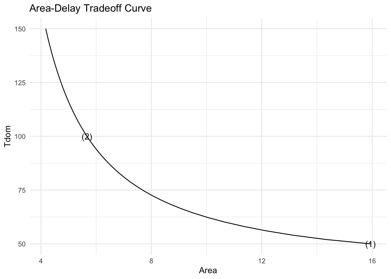

Session Info

R version 4.5.2 (2025-10-31)
Platform: aarch64-apple-darwin20
Running under: macOS Tahoe 26.3

Matrix products: default
BLAS:   /Library/Frameworks/R.framework/Versions/4.5-arm64/Resources/lib/libRblas.0.dylib 
LAPACK: /Library/Frameworks/R.framework/Versions/4.5-arm64/Resources/lib/libRlapack.dylib;  LAPACK version 3.12.1

locale:
[1] en_US.UTF-8/en_US.UTF-8/en_US.UTF-8/C/en_US.UTF-8/en_US.UTF-8

time zone: America/Los_Angeles
tzcode source: internal

attached base packages:
[1] stats     graphics  grDevices datasets  utils     methods   base     

other attached packages:
[1] Matrix_1.7-4    ggplot2_4.0.2   CVXR_1.8.0.9213

loaded via a namespace (and not attached):
 [1] gtable_0.3.6       jsonlite_2.0.0     dplyr_1.2.0        compiler_4.5.2    
 [5] highs_1.12.0-3     tidyselect_1.2.1   Rcpp_1.1.1         dichromat_2.0-0.1 
 [9] scales_1.4.0       yaml_2.3.12        fastmap_1.2.0      clarabel_0.11.2   
[13] lattice_0.22-9     R6_2.6.1           labeling_0.4.3     generics_0.1.4    
[17] knitr_1.51         htmlwidgets_1.6.4  backports_1.5.0    checkmate_2.3.4   
[21] tibble_3.3.1       osqp_1.0.0         pillar_1.11.1      RColorBrewer_1.1-3
[25] rlang_1.1.7        xfun_0.56          S7_0.2.1           otel_0.2.0        
[29] cli_3.6.5          withr_3.0.2        magrittr_2.0.4     digest_0.6.39     
[33] grid_4.5.2         gmp_0.7-5.1        lifecycle_1.0.5    scs_3.2.7         
[37] vctrs_0.7.1        evaluate_1.0.5     glue_1.8.0         farver_2.1.2      
[41] rmarkdown_2.30     pkgconfig_2.0.3    tools_4.5.2        htmltools_0.5.9