n <- 20   # input dimension
m <- 10   # output dimension
N <- 100  # number of training pairs
N_val <- 50  # number of validation pairs

set.seed(243)

## True parameters
A_true <- matrix(rnorm(m * n), nrow = m, ncol = n) / 10
c_true <- abs(rnorm(m))Structured Prediction
Introduction
In this example, we fit a regression model to structured data, using a log-log convex program (LLCP). The training dataset \(\mathcal{D}\) contains \(N\) input-output pairs \((x, y)\), where \(x \in \mathbf{R}^{n}_{++}\) is an input and \(y \in \mathbf{R}^{m}_{++}\) is an output. The entries of each output \(y\) are sorted in ascending order, meaning \(y_1 \leq y_2 \leq \cdots \leq y_m\).
Our regression model \(\phi : \mathbf{R}^{n}_{++} \to \mathbf{R}^{m}_{++}\) takes as input a vector \(x \in \mathbf{R}^{n}_{++}\), and solves an LLCP to produce a prediction \(\hat{y} \in \mathbf{R}^{m}_{++}\). In particular, the solution of the LLCP is the model’s prediction. The model is of the form
\[ \begin{array}{lll} \phi(x) = & \text{argmin} & \mathbf{1}^T (z/y + y/z) \\ & \text{subject to} & y_i \leq y_{i+1}, \quad i = 1, \ldots, m-1 \\ && z_i = c_i x_1^{A_{i1}} x_2^{A_{i2}} \cdots x_n^{A_{in}}, \quad i = 1, \ldots, m. \end{array} \]
Here, the minimization is over \(y \in \mathbf{R}^{m}_{++}\) and an auxiliary variable \(z \in \mathbf{R}^{m}_{++}\), \(\phi(x)\) is the optimal value of \(y\), and the parameters are \(c \in \mathbf{R}^{m}_{++}\) and \(A \in \mathbf{R}^{m \times n}\). The ratios in the objective are meant elementwise. Given a vector \(x\), this model finds a sorted vector \(\hat{y}\) whose entries are close to monomial functions of \(x\) (which are the entries of \(z\)), as measured by the fractional error.
The training loss \(\mathcal{L}(\phi)\) of the model on the training set is the mean squared loss
\[ \mathcal{L}(\phi) = \frac{1}{N} \sum_{(x, y) \in \mathcal{D}} \|y - \phi(x)\|_2^2. \]
We fit the parameters \(c\) and \(A\) by an iterative projected gradient descent method on \(\mathcal{L}(\phi)\). In each iteration, we first compute predictions \(\phi(x)\) for each input in the training set; this requires solving \(N\) LLCPs. Next, we evaluate the training loss \(\mathcal{L}(\phi)\). To update the parameters, we compute the gradient \(\nabla \mathcal{L}(\phi)\) of the training loss with respect to the parameters \(c\) and \(A\). This requires differentiating through the solution map of the LLCP.
This example is described in the paper Differentiating through Log-Log Convex Programs.
Data Generation
We generate synthetic data by choosing a true \(A\) and \(c\), generating lognormal inputs, and solving the LLCP with the true parameters to produce sorted outputs.
generate_data <- function(num_points, seed) {
    set.seed(seed)

    ## Generate lognormal inputs
    inputs <- matrix(exp(rnorm(num_points * n)), nrow = num_points, ncol = n)

    ## For each input, solve the LLCP with true parameters to get output
    input_p <- Parameter(n, pos = TRUE)
    prediction <- c_true * gmatmul(A_true, input_p)
    y_var <- Variable(m, pos = TRUE)
    obj_fn <- sum_entries(prediction / y_var + y_var / prediction)
    cons <- lapply(seq_len(m - 1), function(i) y_var[i] <= y_var[i + 1])
    prob <- Problem(Minimize(obj_fn), cons)

    outputs <- matrix(0, nrow = num_points, ncol = m)
    for (i in seq_len(num_points)) {
        value(input_p) <- inputs[i, ]
        psolve(prob, solver = "SCS", gp = TRUE)
        outputs[i, ] <- value(y_var)
    }
    list(inputs = inputs, outputs = outputs)
}
train_data <- generate_data(N, 243)
train_inputs <- train_data$inputs
train_outputs <- train_data$outputsggplot(data.frame(i = seq_len(m), y = as.vector(train_outputs[1, ])),
aes(i, y)) +
geom_line() + geom_point(size = 2) +
labs(x = "i", y = expression(y[i]),
title = "First Training Output (sorted)") +
theme_minimal()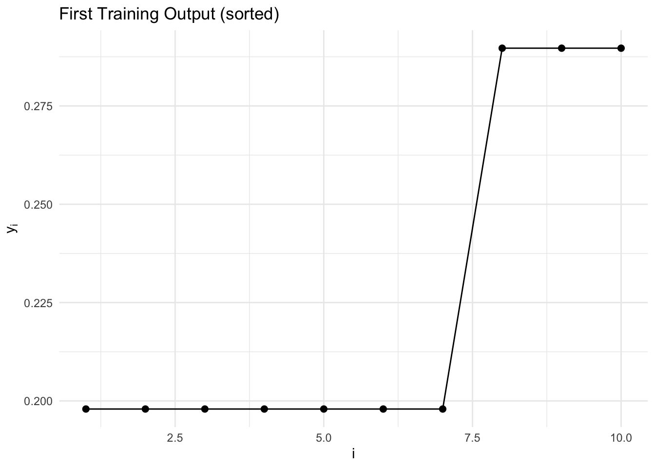
val_data <- generate_data(N_val, 0)
val_inputs  <- val_data$inputs
val_outputs <- val_data$outputs
Monomial Fit to Each Component
We initialize the parameters in our LLCP model by fitting monomials to the training data, without enforcing the monotonicity constraint. This is a standard least squares problem in log space.
log_outputs <- t(log(train_outputs))  # m x N
log_inputs  <- t(log(train_inputs))   # n x N

## Solve: log_outputs ≈ theta^T %*% log_inputs + log_c %*% ones^T
## Variables: theta (n x m), log_c (m x 1)
theta <- Variable(c(n, m))
log_c <- Variable(c(m, 1))
offsets <- do.call(hstack, replicate(N, log_c, simplify = FALSE))  # m x N
cp_preds <- t(theta) %*% log_inputs + offsets   # m x N
lstsq_obj <- (1 / N) * sum_squares(cp_preds - log_outputs)
lstsq_problem <- Problem(Minimize(lstsq_obj))

lstsq_result <- psolve(lstsq_problem, solver = "OSQP", verbose = TRUE)
────────────────────────────────── CVXR v1.9.1 ─────────────────────────────────ℹ Problem: 2 variables, 0 constraints (QP)ℹ Compilation: "OSQP" via CVXR::Dcp2Cone -> CVXR::CvxAttr2Constr -> CVXR::ConeMatrixStuffing -> CVXR::OSQP_QP_Solverℹ Compile time: 0.024s─────────────────────────────── Numerical solver ───────────────────────────────-----------------------------------------------------------------
OSQP v1.0.0 - Operator Splitting QP Solver
(c) The OSQP Developer Team
-----------------------------------------------------------------
problem: variables n = 1210, constraints m = 1000
nnz(P) + nnz(A) = 23000
settings: algebra = Built-in,
OSQPInt = 4 bytes, OSQPFloat = 8 bytes,
linear system solver = QDLDL v0.1.8,
eps_abs = 1.0e-05, eps_rel = 1.0e-05,
eps_prim_inf = 1.0e-04, eps_dual_inf = 1.0e-04,
rho = 1.00e-01 (adaptive: 50 iterations),
sigma = 1.00e-06, alpha = 1.60, max_iter = 10000
check_termination: on (interval 25, duality gap: on),
time_limit: 1.00e+10 sec,
scaling: on (10 iterations), scaled_termination: off
warm starting: on, polishing: on,
iter objective prim res dual res gap rel kkt rho time
1 0.0000e+00 2.49e+00 1.04e+04 -1.58e+05 1.04e+04 1.00e-01 9.59e-04s
50 3.8327e-02 4.41e-09 1.41e-07 2.13e-06 2.13e-06 1.00e-01 2.56e-03s
plsh 3.8327e-02 1.29e-15 1.06e-14 -2.57e-15 1.06e-14 -------- 3.30e-03s
status: solved
solution polishing: successful
number of iterations: 50
optimal objective: 0.0383
dual objective: 0.0383
duality gap: -2.5674e-15
primal-dual integral: 1.5805e+05
run time: 3.30e-03s
optimal rho estimate: 8.90e-04──────────────────────────────────── Summary ───────────────────────────────────✔ Status: optimal✔ Optimal value: 0.0383269ℹ Compile time: 0.024sℹ Solver time: 0.005scat(sprintf("Least squares fit: %f\n", lstsq_result))Least squares fit: 0.038327## Extract initialized parameters
A_init <- t(value(theta)) # m x n
c_init <- exp(value(log_c)) # m x 1Fitting with the LLCP Model
We now set up the parameterized LLCP and iteratively fit the parameters using gradient descent with the backward method.
A_param <- Parameter(c(m, n))
c_param <- Parameter(m, pos = TRUE)
x_slack <- Variable(n, pos = TRUE)
x_param <- Parameter(n, pos = TRUE)
y <- Variable(m, pos = TRUE)

prediction <- c_param * gmatmul(A_param, x_slack)
obj_fn <- sum_entries(prediction / y + y / prediction)
cons <- c(list(x_slack == x_param),
          lapply(seq_len(m - 1), function(i) y[i] <= y[i + 1]))
problem <- Problem(Minimize(obj_fn), cons)

cat(sprintf("Is DGP: %s\n", is_dgp(problem)))
Is DGP: TRUEWe run projected gradient descent. In each epoch, for every training example, we solve the LLCP, compute the gradient of the squared loss with respect to \(A\) and \(c\) via backward, and accumulate the gradients. We then update the parameters.
## Initialize parameters from the monomial fit
A_current <- A_init
c_current <- as.vector(c_init)

lr <- 5e-2  # learning rate
n_epochs <- 10

train_losses <- numeric(n_epochs)
val_losses   <- numeric(n_epochs)

for (epoch in seq_len(n_epochs)) {
    ## -- Training pass --
    A_grad_accum <- matrix(0, m, n)
    c_grad_accum <- numeric(m)
    train_loss <- 0

    for (i in seq_len(N)) {
        value(A_param) <- A_current
        value(c_param) <- c_current
        value(x_param) <- train_inputs[i, ]

        psolve(problem, gp = TRUE, requires_grad = TRUE, solve_method = "SCS")
        y_pred <- value(y)
        residual <- y_pred - train_outputs[i, ]
        train_loss <- train_loss + sum(residual^2)

        ## Set gradient of y to d(loss)/d(y) = 2 * residual / N
        gradient(y) <- 2 * residual / N
        backward(problem)

        A_grad_accum <- A_grad_accum + gradient(A_param)
        c_grad_accum <- c_grad_accum + gradient(c_param)
    }
    train_losses[epoch] <- train_loss / N

    ## -- Validation pass (no gradients needed) --
    val_loss <- 0
    for (i in seq_len(N_val)) {
        value(A_param) <- A_current
        value(c_param) <- c_current
        value(x_param) <- val_inputs[i, ]
        psolve(problem, solver = "SCS", gp = TRUE)
        y_pred <- value(y)
        val_loss <- val_loss + sum((y_pred - val_outputs[i, ])^2)
    }
    val_losses[epoch] <- val_loss / N_val

    cat(sprintf("(epoch %d) train / val (%.4f / %.4f)\n",
                epoch, train_losses[epoch], val_losses[epoch]))

    ## -- Update parameters --
    A_current <- A_current - lr * A_grad_accum
    c_current <- c_current - lr * c_grad_accum
    ## Project c to stay positive
    c_current <- pmax(c_current, 1e-8)
}
(epoch 1) train / val (0.0013 / 0.0022)
(epoch 2) train / val (0.0013 / 0.0022)
(epoch 3) train / val (0.0013 / 0.0022)
(epoch 4) train / val (0.0012 / 0.0022)
(epoch 5) train / val (0.0012 / 0.0022)
(epoch 6) train / val (0.0012 / 0.0022)
(epoch 7) train / val (0.0012 / 0.0022)
(epoch 8) train / val (0.0012 / 0.0022)
(epoch 9) train / val (0.0012 / 0.0022)
(epoch 10) train / val (0.0012 / 0.0022)Comparing Predictions
We compare the LLCP model predictions (with fitted parameters) to the true outputs on a validation example.
## Compute LLCP predictions on a validation example
val_idx <- 1
value(A_param) <- A_current
value(c_param) <- c_current
value(x_param) <- val_inputs[val_idx, ]
psolve(problem, solver = "SCS", gp = TRUE)
[1] 20.00638llcp_pred <- as.vector(value(y))
## Compute least-squares monomial predictions (no monotonicity)
lstsq_pred <- as.vector(as.vector(c_init) *
exp(A_init %*% log(val_inputs[val_idx, ])))
pred_df <- data.frame(
i = rep(seq_len(m), 3),
y = c(as.vector(val_outputs[val_idx, ]), llcp_pred, lstsq_pred),
series = factor(rep(c("True", "LLCP", "Least Squares"), each = m),
levels = c("True", "LLCP", "Least Squares")))
ggplot(pred_df, aes(i, y, color = series, shape = series)) +
geom_line() + geom_point(size = 2) +
scale_color_manual(values = c("True" = "orange", "LLCP" = "#008080",
"Least Squares" = "gray")) +
labs(x = "i", y = expression(y[i]), color = NULL, shape = NULL,
title = "Validation Example: True vs. Predictions") +
theme_minimal() + theme(legend.position = "top")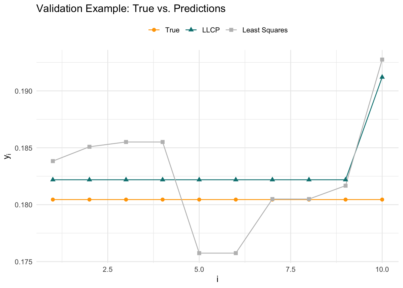
Session Info
R version 4.6.0 (2026-04-24)
Platform: aarch64-apple-darwin23
Running under: macOS Tahoe 26.5.1

Matrix products: default
BLAS:   /Library/Frameworks/R.framework/Versions/4.6/Resources/lib/libRblas.0.dylib
LAPACK: /Library/Frameworks/R.framework/Versions/4.6/Resources/lib/libRlapack.dylib;  LAPACK version 3.12.1

locale:
[1] en_US.UTF-8/en_US.UTF-8/en_US.UTF-8/C/en_US.UTF-8/en_US.UTF-8

time zone: America/Los_Angeles
tzcode source: internal

attached base packages:
[1] stats     graphics  grDevices utils     datasets  methods   base

other attached packages:
[1] ggplot2_4.0.3 CVXR_1.9.1

loaded via a namespace (and not attached):
 [1] Matrix_1.7-5       gtable_0.3.6       jsonlite_2.0.0     dplyr_1.2.1
 [5] compiler_4.6.0     highs_1.14.0-2     tidyselect_1.2.1   Rcpp_1.1.1-1.1
 [9] dichromat_2.0-0.1  scales_1.4.0       yaml_2.3.12        fastmap_1.2.0
[13] clarabel_0.11.2    lattice_0.22-9     R6_2.6.1           labeling_0.4.3
[17] generics_0.1.4     knitr_1.51         htmlwidgets_1.6.4  backports_1.5.1
[21] checkmate_2.3.4    tibble_3.3.1       osqp_1.0.0         pillar_1.11.1
[25] RColorBrewer_1.1-3 rlang_1.2.0        xfun_0.58          S7_0.2.2
[29] otel_0.2.0         cli_3.6.6          withr_3.0.2        magrittr_2.0.5
[33] digest_0.6.39      grid_4.6.0         gmp_0.7-5.1        lifecycle_1.0.5
[37] scs_3.2.7          vctrs_0.7.3        diffcp_0.1.1       evaluate_1.0.5
[41] glue_1.8.1         farver_2.1.2       rmarkdown_2.31     pkgconfig_2.0.3
[45] tools_4.6.0        htmltools_0.5.9