Consider a triangle, or a wedge, located within a hypersonic flow. A standard aerospace design optimization problem is to design the wedge to maximize the lift-to-drag ratio (L/D) (or conversely minimize the D/L ratio), subject to certain geometric constraints. In this example, the wedge is known to have a constant hypotenuse, and our job is to choose its width and height.
Problem Formulation
The drag-to-lift ratio is given by
\[
\frac{D}{L} = \frac{c_d}{c_l},
\]
where \(c_d\) and \(c_l\) are drag and lift coefficients, respectively, that are obtained by integrating the projection of the pressure coefficient in directions parallel to, and perpendicular to, the body.
We will assume the pressure coefficient is given by the Newtonian sine-squared law for whetted areas of the body,
\[
c_p = 2(\hat{v} \cdot \hat{n})^2
\]
and elsewhere \(c_p = 0\). Here, \(\hat{v}\) is the free stream direction, which for simplicity we assume is parallel to the body so that \(\hat{v} = \langle 1, 0 \rangle\), and \(\hat{n}\) is the local unit normal. For a wedge defined by width \(\Delta x\) and height \(\Delta y\),
\[
\hat{n} = \langle -\Delta y / s, -\Delta x / s \rangle
\]
This function is representable as a DQCP quasilinear function.
Plotting the Objective
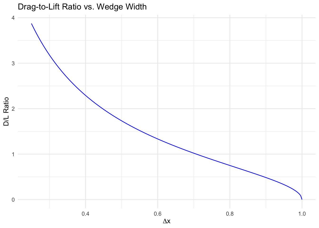
We can visualize the D/L ratio as a function of \(\Delta x\):
x_vals <-seq(0.25, 1, length.out =201)obj_vals <-sqrt(1/ x_vals^2-1)ggplot(data.frame(x = x_vals, y = obj_vals), aes(x, y)) +geom_line(color ="blue") +labs(x =expression(Delta * x), y ="D/L Ratio",title ="Drag-to-Lift Ratio vs. Wedge Width") +theme_minimal()
DQCP Formulation
We now express the objective in CVXR and verify its curvature:
x <-Variable(pos =TRUE)obj <-sqrt(inv_pos(power(x, 2)) -1)cat("This objective function is", curvature(obj), "\n")
This objective function is QUASILINEAR
Minimizing this objective function subject to constraints representing payload requirements is a standard aerospace design problem. In this case we consider the constraint that the wedge must be able to contain a rectangle of given length and width internally along its hypotenuse. This is representable as a convex constraint.
a <-0.05# height of rectangle (should be at most b)b <-0.65# width of rectangleconstraint <-list(a *inv_pos(x) - (1- b) *sqrt(1-power(x, 2)) <=0)
Warning: Solution may be inaccurate. Try another solver, adjusting the solver settings,
or solve with `verbose = TRUE` for more information.
Solution may be inaccurate. Try another solver, adjusting the solver settings,
or solve with `verbose = TRUE` for more information.
Solution may be inaccurate. Try another solver, adjusting the solver settings,
or solve with `verbose = TRUE` for more information.
check_solver_status(prob)ld_ratio <-1/ resultx_opt <-value(x)y_opt <-sqrt(1- x_opt^2)cat("Final L/D Ratio:", ld_ratio, "\n")cat("Final width of wedge:", x_opt, "\n")cat("Final height of wedge:", y_opt, "\n")
Final L/D Ratio: 6.854065
Final width of wedge: 0.9895237
Final height of wedge: 0.1443703
Verification Plot
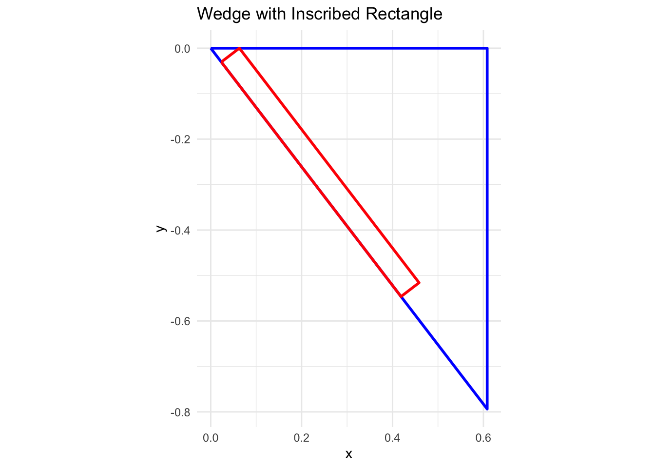
Once the solution has been found, we can create a plot to verify that the rectangle is inscribed within the wedge.
y <-sqrt(1- x_opt^2)lambda1 <- a * x_opt / y## Wedge verticeswedge <-data.frame(x =c(0, x_opt, x_opt, 0),y =c(0, 0, -y, 0))## Rectangle verticespt1 <-c(lambda1 * x_opt, -lambda1 * y)pt2 <-c((lambda1 + b) * x_opt, -(lambda1 + b) * y)pt3 <-c((lambda1 + b) * x_opt + a * y, -(lambda1 + b) * y + a * x_opt)pt4 <-c(lambda1 * x_opt + a * y, -lambda1 * y + a * x_opt)rect <-data.frame(x =c(pt1[1], pt2[1], pt3[1], pt4[1], pt1[1]),y =c(pt1[2], pt2[2], pt3[2], pt4[2], pt1[2]))ggplot() +geom_path(data = wedge, aes(x, y), color ="blue", linewidth =1) +geom_path(data = rect, aes(x, y), color ="red", linewidth =1) +coord_fixed() +labs(title ="Wedge with Inscribed Rectangle") +theme_minimal()